
Il rapporto Gabriel 1996
Compilation of the dielectric properties of body tissues at RF and microwave frequencies
Camelia Gabriel, PhD and Sami Gabriel, MSc — Physics Department, King's College London, London WC2R 2LS, UK.
Report AL/OE-TR-1996-0037, June 1996. Final report for the period 15 December 1994 – 14 December 1995, prepared for AFOSR/NL Bolling AFB DC 20332-0001. Armstrong Laboratory (AFMC), Occupational and Environmental Health Directorate, Radiofrequency Radiation Division, Brooks Air Force Base, TX 78235-5102.
Approvato per la diffusione pubblica, senza limitazioni
(DTIC AD-A305826). La scheda Rapporto
contiene il rapporto stesso; i dati a cui si
riferisce stanno nelle altre schede, presi dal database invece che dalle 390 immagini
del documento originale.
Introduction
Recent developments in the field of electromagnetic dosimetry have produced high resolution anatomically correct man and animal models from medical imaging data for use in numerical simulation exercises. The level of detail is such that over 30 tissue types can be identified. The application of such models requires that dielectric properties be allocated to the various tissues at all the frequencies to which the model is exposed. There is, as yet, no consensus on the dielectric data. This project is geared towards this objective. The following has been achieved in the period covered by this report:
- Three experimental techniques were used to measure the dielectric properties of tissue in the frequency range 10 Hz to 20 GHz. Over 20 tissue types were measured over the full frequency range and over 10 others measured down to 1 MHz only.
- Internal consistency between the three sets of data was demonstrated in the overlapping frequency regions. When measurements are made on the same sample throughout, the agreement between data sets is particularly good.
- A comprehensive survey of dielectric data published over more than 45 years has been carried out and presented for comparison purposes. The data obtained in the course of this study fall well within the vast body of literature data where available, and bridge the gaps within it.
- To facilitate the incorporation of the dielectric data in numerical solutions, their frequency dependence was modelled to a spectrum characterised by 4 dispersion regions. This model was successfully applied to the new experimental data.
- Finally, the conductivity of tissues below 100 Hz was estimated from the recent measurements mitigated by data from the literature and used to estimate the conductivity of the whole body and of various body parts.
The work is briefly described in this report; the data are presented in graphical and tabular format in the Experimental data tab, graphs and numbers together (Appendices A to D of the original document).
Experimental techniques
Techniques
The dielectric measurements were performed using automatic swept frequency network and impedance analysers. For the frequency range 10 Hz to 10 MHz, an HP4192A impedance analyser. An HP 8753C covered the frequency range 300 kHz to 3 GHz and an HP8720 measured from 130 MHz to 20 GHz. Open ended coaxial probes were used to interface the measuring equipment with the samples in all cases. The technique used with the HP8700 series network analysers has been reported in detail elsewhere (Gabriel et al 1994) and will not be discussed further. The techniques used in conjunction with the impedance analyser will be briefly described.
A 50 ohm impedance matched conical coaxial probe was adapted (Gabriel and Grant 1988) to interface the sample to the HP4192A impedance analyser. The probe is characterised by a fringing capacitance C and conductance G which are a function of its physical dimension and can be measured with the impedance analyser. The characteristic parameters of the probe were calculated from measurements of the impedance components of the probe in air and in a standard sample (water or salt solution). In principle, the dielectric properties (permittivity and conductivity ) of an unknown sample can then be calculated from measurements of the impedance of the probe against an unknown sample using the following relationships, where is the permittivity of free space and the probe constant:
(1)
In practice, the measurement of conductive materials in the frequency range 10 Hz to 10 MHz is not so straightforward. The measurements are affected by two sources of systematic errors, electrode polarisation and lead inductance errors, which become apparent at the lower and higher ends of the frequency range under consideration. Electrode polarisation is a manifestation of molecular charge organisation which occurs at the sample–electrode interface in the presence of water molecules and hydrated ions. In its simplest form the phenomenon is equivalent to a frequency dependent capacitor in series with a resistor. Both components can be approximated by negative power functions of frequency, that is their absolute values decrease with increasing frequency. The effect increases with increasing sample conductivity and its consequences are more pronounced on the capacitance than the conductance of ionic solutions as well as biological samples (Schwan 1992). In the case of biological samples, the poorly conducting cells shield part of the electrode from the ionic current thus reducing the polarisation effects compared to an ionic solution equivalent in conductivity to the intracellular fluid.
The material of the electrode plays an important part in determining its polarisation impedance. In the current study gold plated and sputtered platinum electrodes were tested and a choice was made in favour of the latter. The effect of the rough platinum surface was to shift the electrode polarisation effect to lower frequencies and thus to reduce its contribution in the frequency range under consideration.
The inductance of the probe and connecting cable adds another series component to the measured impedance. Its value could be determined from measurements on standard salt solutions and applying an equivalent circuit analysis. For the present setup the stray inductance is and the following equations were used to account for it:
(2)
where C and G are the corrected capacitance and conductance expressed in terms of the measured values and , the lead inductance L and the angular frequency . The effect of the stray inductance increases with frequency and with sample conductivity.
Figures 1a and 1b show the effect of electrode polarisation and the stray inductance on the uncorrected permittivity and conductivity of a series of salt solutions ranging from zero molar (deionised water) to 0.09 molar. The high permittivity values at low frequencies are a manifestation of electrode polarisation, while negative permittivity values at high frequency show the effect of the stray inductance. Superimposed on these data are the uncorrected permittivity and conductivity of a tissue sample (heart tissue). It can be seen that the low frequency conductivity of the tissue is less than that of 0.01 molar salt solution. It is therefore reasonable to assume that the effect of electrode polarisation on the tissue is also less than that exhibited by the 0.01 molar salt sample. A further observation indicates that the errors in the permittivity and conductivity of the sample are likely to be apparent below 1 kHz and significant below 100 Hz, while the effect of inductance manifests above a few megahertz in the case of tissue samples.
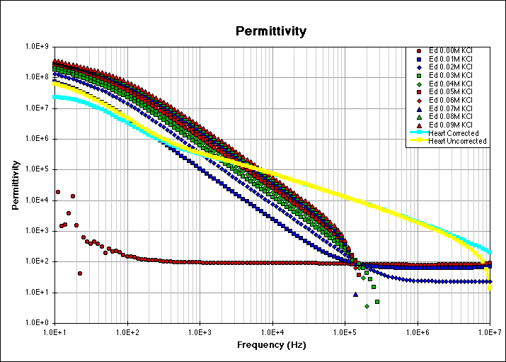
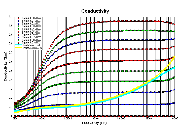
Figure 1. Uncorrected values of the permittivity and conductivity of a series of salt solutions. Also shown are the corrected and uncorrected data for heart tissue at 37 °C.
Delle dodici serie della figura, due sono nel database e si possono esplorare qui sotto: Heart corrected, che è la serie misurata dell'appendice D, e Heart uncorrected, letta dai pixel di questa figura (scarto mediano 3%). Il confronto fra le due è l'effetto della polarizzazione degli elettrodi, che è quello che la figura vuole mostrare. Le dieci soluzioni di KCl restano visibili soltanto nell'immagine.
Costruzione del grafico dai dati del rapporto…
To correct for electrode polarisation and induction errors, the capacitance and conductance of the tissue sample are evaluated in accordance with (2) and normalised to a salt solution of similar low frequency conductivity. The example in Figures 1a and 1b was corrected with reference to a 0.005 molar salt solution; the corrected dielectric properties are shown for comparison purposes. All impedance analyser tissue measurements were treated in a similar manner.
Uncertainties
The measurement techniques and associated instrumentation used in this study give random reproducibility of about 1% across the frequency range. This statement is based on multiple measurements carried out on standard samples of uniform composition. Biological tissues are inhomogeneous and show considerable variability in structure or composition and hence in dielectric properties. Such variations are natural and may be due to physiological processes or other functional requirements. The spread of values ranges from about ±5% above 100 MHz to ±15% at the lower end of the frequency scale. Care has been taken to eliminate all known sources of systematic errors; however, in view of the assumptions made in correcting for electrode polarisation it is possible that the dielectric parameters below 1 kHz may be undercorrected. This source of errors may affect the dielectric parameters by up to a factor of two.
Materials
Three sources of materials were used: excised animal tissue, mostly ovine, from freshly killed sheep; human autopsy materials; human skin and tongue in vivo. All animal tissues were used as fresh as possible, mostly within two hours of death; human material was obtained 24 to 48 hours after death. The conical probe used in conjunction with the impedance analyser requires relatively large samples, at least a cube of 5 cm linear dimension. In view of this requirement not all samples could be measured at low frequencies.
Results
Measurements across the frequency range
Examples of measurements on the three experimental setups, across the frequency range, are given in the Experimental data tab: where a tissue was measured with more than one instrument, each run appears as a separate series. The agreement between measurements on the three machines was particularly good when the measurements were made on the same sample throughout. To achieve this objective the two network analysers and the impedance analyser were placed in close proximity to each other and interfaced to the same computer. All the measurement procedures were redesigned to operate through LabView, a graphics interface medium from National Instruments running on an Intel Pentium microprocessor. In this arrangement, the measurements could be carried out on all three machines in quick succession.
The dielectric properties of muscle are known to be anisotropic. The data reported were obtained by measurement on the paravertebral muscle. The sample was measured twice, first with a transverse section against the probe and then it was cut along the muscle fibre and re-measured. In view of the radial nature of the fringing field of the coaxial probe these measurements do not represent the true limits of the dielectric properties with the field along and across the fibre. They show, however, the effect of fibre direction and the parts of the spectrum influenced by it.
Human material could not be obtained in sufficient quantities for optimum measurements with the conical probe. Under such conditions the measurements on the impedance analyser were consistently lower than those obtained on the network analyser in the same frequency range. Much smaller samples of human material were measured only in the frequency range above 1 MHz on the two impedance analysers.
Comparison between species
The differences in the dielectric properties of animal and human species are not systematic. The variation in tissue properties within a species may well exceed variations between species. Examples of comparative measurements are given in Figures 2 to 4.
Costruzione del grafico dai dati del rapporto…
Grafico ricostruito dal database. La serie Human @ 37 °C viene dall'appendice D del rapporto; le altre due sono state lette dai pixel della figura originale, perché il rapporto non le tabula: scarto mediano 0,8%, misurato digitalizzando nella stessa figura la serie di cui i valori veri sono noti.
Costruzione del grafico dai dati del rapporto…
Grafico ricostruito dal database. La serie Bovine @ 37 °C viene dall'appendice D; quella ovina è stata letta dai pixel della figura originale: scarto mediano 1,2%.
Costruzione del grafico dai dati del rapporto…
Grafico ricostruito dal database. La serie Human @ 37 °C viene dall'appendice D; quella ovina a 30 °C è stata letta dai pixel della figura originale: scarto mediano 0,8%.
Le figure 2, 3 e 4 sono ora grafici costruiti dal database: la serie che il rapporto tabula e quelle che mostrava solo nel disegno, lette dai pixel e riconoscibili dal colore violetto. La figura 1 resta un'immagine, perché delle sue dodici serie dieci sono soluzioni di KCl disegnate con tre soli colori e marcatori sovrapposti: separarle non è possibile, e dove un marcatore copre l'altro il dato sottostante non esiste più.
Literature survey
Review of the dielectric properties of tissues
The dielectric properties of tissues have been extracted from the literature of the past five decades and compared to the corresponding data from the current study. The purpose is to provide an objective basis for the evaluation of the experimental data and to reach a broad based consensus on the subject. Reports of dielectric properties of tissues prior to 1950 are difficult to get hold of; they have more historical than practical interest and, with the exception of Osswald (1937), have not been reviewed. The literature in the 1950s and 60s is dominated by the work of H. P. Schwan and his collaborators and has been reviewed and tabulated by Durney et al 1986. Other extensive reviews include Geddes and Baker (1967), who summarised the early reports on the specific resistance of tissues; Stuchly and Stuchly (1980), who tabulated the dielectric properties of tissues in the frequency range 10 kHz to 10 GHz; Foster and Schwan (1989), who provided a wide historical perspective; and Duck (1990), who extended their survey by including more recent data.
In the current survey, data that correspond more closely to living human tissues were selected in preference to any other. Consequently, human tissue and in vivo measurements were selected in preference to animal tissue and in vitro measurements. For in vitro measurements, data obtained at temperatures closest to that of the body and nearest to the time after death were used when available. Most of the literature data were in graphical rather than table form and in a logarithmic rather than linear format. Such data were retrieved at each decade. When tables were available, a more extensive frequency range was often provided. The data were translated from the various authors' preferred set of parameters and units to relative permittivity and conductivity expressed in S/m.
Data obtained at temperatures as low as 20 °C are included in this survey. It was not considered advisable to translate them to body temperature. The temperature coefficients, for both permittivity and conductivity, are tissue-type and frequency dependent. Information on these coefficients is scarce and not sufficiently robust to warrant generalisation and extrapolation. Moreover, the coefficients are highest (~1–2 %/°C) at low frequencies where the uncertainty and the scatter in the data are of a similar or higher order of magnitude than the differences due to 10 or 15 °C.
Presentation of data
Details of the tissue type, animal species, measurement temperature and the reference are included with each series: in this page they appear in the legend of the graph and in the table below it, so that every literature point can be traced to the paper it came from.
Data analysis
Parametric description of the dielectric spectrum
One of the aims of this project is to derive models for the frequency dependence of the dielectric properties of the tissues investigated. The basis of the analysis is the well known dispersions in the dielectric spectrum of biological materials and their expression as a summation of terms corresponding to the main polarisation mechanisms. The spectrum extends from Hz to GHz and shows 4 dispersion regions. The complexity of the structure and composition of biological material is such that each dispersion region is broadened by multiple contributions to it and could be described by a Cole-Cole expression. The model corresponding to the whole spectrum is:
(3)
in which is the permittivity in the terahertz frequency range, is the ionic conductivity and, for each dispersion region, is the relaxation time, the broadening parameter and the drop in permittivity in the frequency range corresponding to .
With a choice of parameters appropriate to each tissue, (3) can be used to predict its dielectric behaviour over the desired frequency range. The parameters of the model were adjusted to correspond to a close fit between the model and the most comprehensive data set available for the particular tissue. The 4-Cole-Cole model describes the frequency dependence of the dielectric properties in the frequency range from Hz to GHz. It can be used with confidence for frequencies above 1 MHz. At lower frequencies, where the literature values are scarce and have larger than average uncertainties, the model should be used with caution in the knowledge that it provides a best estimate based on present knowledge. It is important to stress the limitations of the model, particularly where there are no data at all to support its predictions. The 4-Cole-Cole analysis was carried out on 44 tissue types; the resulting parameters are in the Model parameters tab, and the experimental data they were fitted to in the Experimental data tab.
The dielectric properties below 100 Hz
Electrical properties of body tissues
Below 100 Hz the impedance of biological material is mostly resistive. The contribution of the capacitive component is of the order of 10% in most cases. The literature surveyed in this study shows that there are wide variations in the conductivity values obtained for the same tissue in various studies. The contribution of the tissue permittivity to body current is well within the uncertainty associated with the corresponding tissue conductivity. Therefore, in practice, the estimation of induced current in tissue is based on such conductivity values. Table 1 gives an estimate for conductivity in S/m of the main body tissues below 100 Hz from this study, mitigated by literature values. The values tabulated by Duck (1990) are also shown for comparison. Average values were used where appropriate.
Table 1. Estimates of the conductivity (S/m) of body tissues below 100 Hz at body temperature.
| Tissue | From Duck 1990 | This study |
|---|---|---|
| Bladder | — | 0.2 |
| Blood | 0.68 | 0.7 |
| Bone -Cancellous | — | 0.07 |
| Bone -Cortical | 0.02 | 0.02 |
| Bone -Marrow | — | 0.05 |
| Breast | — | 0.06 |
| Cartilage | — | 0.18 |
| Cerebellum | — | 0.1 |
| Cerebro Spinal Fluid | 1.81 | 2 |
| Colon | — | 0.1 |
| Cornea | — | 0.4 |
| Dura | — | 0.5 |
| Fat | — | 0.04 |
| Gall Bladder Bile | 1.6 | 1.4 |
| Grey Matter | 0.3 | 0.1 |
| Heart | 0.2 | 0.1 |
| Kidney | 0.9 | 0.1 |
| Lens | — | 0.25 |
| Liver | 0.12 | 0.07 |
| Lung -Deflated | 0.1 | 0.2 |
| Lung -Inflated | 0.05 | 0.08 |
| Muscle | 0.4 | 0.35 |
| Nerve | 0.4 | 0.03 |
| Pancreas | 0.13 | 0.22 |
| Skin -Wet | — | 0.1 |
| Small Intestine | — | 0.5 |
| Spleen | — | 0.1 |
| Stomach | — | 0.5 |
| Tendon | — | 0.3 |
| Testis | — | 0.4 |
| Thyroid | — | 0.5 |
| Tongue | — | 0.3 |
| Urine | 3.3 | — |
| Vitreous Humour | — | 1.5 |
| White matter | 0.1 | 0.06 |
Electrical properties of body parts
The values obtained from this study were used to calculate the conductivity of the whole and various parts of the body (Table 2). The necessary integration of the conductivity of tissue to obtain the values in Table 2 was carried out by allocating the appropriate values to a voxel anatomical human model developed at the National Radiological Protection Board (NRPB) to aid dosimetry work. The model, known as NORMAN (normal man), will be described in a future NRPB publication. The results of such an integration carried out at 10 and 100 kHz have also been included for comparison purposes.
Table 2. Conductivity, in S/m, of the whole body and parts of the body, obtained by integrating the conductivity values of Table 1 over various parts of the body.
| Frequency | Whole body | Head | Torso | Arm | Leg | Neck |
|---|---|---|---|---|---|---|
| 50 Hz | 0.216 | 0.254 | 0.223 | 0.195 | 0.196 | — |
| 10 kHz | 0.276 | 0.285 | 0.256 | — | 0.238 | 0.222 |
| 100 kHz | 0.288 | 0.3 | 0.332 | — | 0.239 | 0.243 |
Conclusions
The main purpose of this project is to compile a database of dielectric properties of tissues for use by the scientific community in solving electromagnetic interaction problems. This has been achieved through measurement in the frequency range 10 Hz to 20 GHz and modelling the frequency dependence of the dielectric properties of over 30 body tissues to parametric expressions for inclusion in numerical solutions.
References
- C. Gabriel, T. Y. A. Chan and E. H. Grant,
Admittance models for open ended coaxial probes and their place in dielectric spectroscopy
, Physics in Medicine and Biology, 39, 12, 2183–2200, 1994. - C. Gabriel and E. H. Grant,
Dielectric sensors for industrial microwave measurements and control
, Mikrowellen und HF Magazin, 15, 643–645, 1989. - H. P. Schwan,
Linear and nonlinear electrode polarisation and biological materials
, Annals of Biomedical Engineering, 20, 269–288, 1992. - C. H. Durney, H. Massoudi and M. F. Iskander, Radiofrequency radiation dosimetry handbook, Brooks Air Force Base, USAFSAM-TR-85-73, 1986.
- L. A. Geddes and L. E. Baker,
The specific resistance of biological material: a compendium of data for the biomedical engineer and physiologist
, Medical and Biological Engineering, 5, 271–293, 1967. - M. A. Stuchly and S. S. Stuchly,
Dielectric properties of biological substances: tabulated
, Journal of Microwave Power, 15, 1, 19–26, 1980. - K. R. Foster and H. P. Schwan,
Dielectric properties of tissues and biological materials: a critical review
, Critical Reviews in Biomedical Engineering, 17, 1, 25–104, 1989. - F. A. Duck, Physical properties of tissue: a comprehensive reference book, Academic Press, Harcourt Brace Jovanovich, 1990.
Original web edition written by Sami Gabriel, last updated 5 November 1997. Transcribed here with the figures and tables served from the database; the wording of the report is unchanged.
La curva del modello copre tutto il campo che il servizio tratta, da 10 Hz a 100 GHz; i dati sperimentali si fermano a 20 GHz. Dove una tabella del rapporto contiene più campioni di misura, ciascuno diventa una serie a sé: sono le bande di frequenza coperte da sonde diverse.
| Serie | Fonte | Punti | Campo di frequenza (Hz) | Specie e condizioni | Riferimento |
|---|
Permittività, fattore di perdita e conducibilità sono legati da σ = 2πfε0ε″, ma nel rapporto non lo sono sempre: i valori sono riportati come pubblicati, senza correzioni. Nelle tabelle delle misure 63 punti su 6636 sbagliano di oltre il 2% (fino al 16%, nelle bande dove il fattore di perdita salta mentre permittività e conducibilità restano lisce); in quelle di letteratura lo scarto arriva a un fattore dieci. I grafici usano permittività e conducibilità, la coppia che il modello riproduce.
I punti di una serie, nei valori pubblicati dal rapporto. I bottoni salvano la serie con la sua provenienza in testa al file.
I parametri dell'equazione (3) per ciascuno dei 57 tessuti che il servizio conosce: la tabella riassuntiva dell'Appendice C, allargata negli anni con i tessuti aggiunti dal CNR-IFAC. Sono i valori che il calcolo usa davvero, letti dalle stesse righe del database. I tempi di rilassamento sono nei sottomultipli usati dal rapporto.
| Tessuto | ε∞ | σi (S/m) | Δε1 | τ1 (ps) | α1 | Δε2 | τ2 (ns) | α2 | Δε3 | τ3 (µs) | α3 | Δε4 | τ4 (ms) | α4 |
|---|---|---|---|---|---|---|---|---|---|---|---|---|---|---|
| Air | 1 | 0 | 0 | 0 | 1 | 0 | 0 | 1 | 0 | 0 | 1 | 0 | 0 | 1 |
| Aorta | 4 | 0.25 | 40 | 8.842 | 0.1 | 50 | 3.183 | 0.1 | 1.0e+5 | 159.16 | 0.2 | 1.0e+7 | 1.592 | 0 |
| Bladder | 2.5 | 0.2 | 16 | 8.842 | 0.1 | 400 | 159.16 | 0.1 | 1.0e+5 | 159.16 | 0.2 | 1.0e+7 | 15.915 | 0 |
| Blood | 4 | 0.7 | 56 | 8.377 | 0.1 | 5200 | 132.63 | 0.1 | 0 | 159.16 | 0.2 | 0 | 15.915 | 0 |
| Blood vessel | 4 | 0.25 | 40 | 8.842 | 0.1 | 50 | 3.183 | 0.1 | 1.0e+5 | 159.16 | 0.2 | 1.0e+7 | 1.592 | 0 |
| Body fluid | 4 | 1.5 | 65 | 7.234 | 0 | 30 | 159.16 | 0.1 | 0 | 159.16 | 0 | 0 | 15.915 | 0 |
| Bone cancellous | 2.5 | 0.07 | 18 | 13.263 | 0.22 | 300 | 79.577 | 0.25 | 20000 | 159.16 | 0.2 | 2.0e+7 | 15.915 | 0 |
| Bone cortical | 2.5 | 0.02 | 10 | 13.263 | 0.2 | 180 | 79.577 | 0.2 | 5000 | 159.16 | 0.2 | 1.0e+5 | 15.915 | 0 |
| Bone marrow | 2.5 | 0.0005 | 3 | 7.958 | 0.2 | 25 | 15.915 | 0.1 | 5000 | 1591.5 | 0.1 | 2.0e+6 | 15.915 | 0.1 |
| Brain grey matter | 4 | 0.02 | 45 | 7.958 | 0.1 | 400 | 15.915 | 0.15 | 2.0e+5 | 106.1 | 0.22 | 4.5e+7 | 5.305 | 0 |
| Brain white matter | 4 | 0.02 | 32 | 7.958 | 0.1 | 100 | 7.958 | 0.1 | 40000 | 53.052 | 0.3 | 3.5e+7 | 7.958 | 0.02 |
| Breast fat | 2.5 | 0.01 | 3 | 17.68 | 0.1 | 15 | 63.66 | 0.1 | 50000 | 454.7 | 0.1 | 2.0e+7 | 13.26 | 0 |
| Cartilage | 4 | 0.15 | 38 | 13.263 | 0.15 | 2500 | 144.69 | 0.15 | 1.0e+5 | 318.31 | 0.1 | 4.0e+7 | 15.915 | 0 |
| Cerebellum | 4 | 0.04 | 40 | 7.958 | 0.1 | 700 | 15.915 | 0.15 | 2.0e+5 | 106.1 | 0.22 | 4.5e+7 | 5.305 | 0 |
| Cerebro spinal fluid | 4 | 2 | 65 | 7.958 | 0.1 | 40 | 1.592 | 0 | 0 | 159.16 | 0 | 0 | 15.915 | 0 |
| Cervix | 4 | 0.3 | 45 | 7.958 | 0.1 | 200 | 15.915 | 0.1 | 1.5e+5 | 106.1 | 0.18 | 4.0e+7 | 1.592 | 0 |
| Colon | 4 | 0.01 | 50 | 7.958 | 0.1 | 3000 | 159.16 | 0.2 | 1.0e+5 | 159.16 | 0.2 | 4.0e+7 | 1.592 | 0 |
| Cornea | 4 | 0.4 | 48 | 7.958 | 0.1 | 4000 | 159.16 | 0.05 | 1.0e+5 | 15.915 | 0.2 | 4.0e+7 | 15.915 | 0 |
| Duodenum | 4 | 0.5 | 60 | 7.958 | 0.1 | 2000 | 79.577 | 0.1 | 1.0e+5 | 159.16 | 0.2 | 4.0e+7 | 15.915 | 0 |
| Dura | 4 | 0.5 | 40 | 7.958 | 0.15 | 200 | 7.958 | 0.1 | 10000 | 159.16 | 0.2 | 1.0e+6 | 15.915 | 0 |
| Eye sclera | 4 | 0.5 | 50 | 7.958 | 0.1 | 4000 | 159.16 | 0.1 | 1.0e+5 | 159.16 | 0.2 | 5.0e+6 | 15.915 | 0 |
| Fat | 2.5 | 0.01 | 3 | 7.958 | 0.2 | 15 | 15.915 | 0.1 | 33000 | 159.16 | 0.05 | 1.0e+7 | 7.958 | 0.01 |
| Gall bladder | 4 | 0.9 | 55 | 7.579 | 0.05 | 40 | 1.592 | 0 | 1000 | 159.16 | 0.2 | 10000 | 15.915 | 0 |
| Gall bladder bile | 4 | 1.4 | 66 | 7.579 | 0.05 | 50 | 1.592 | 0 | 0 | 159.16 | 0.2 | 0 | 15.915 | 0.2 |
| Gland | 4 | 0.5 | 55 | 7.958 | 0.1 | 2500 | 159.16 | 0.1 | 1.0e+5 | 159.16 | 0.2 | 4.0e+7 | 15.915 | 0 |
| Heart | 4 | 0.05 | 50 | 7.958 | 0.1 | 1200 | 159.16 | 0.05 | 4.5e+5 | 72.343 | 0.22 | 2.5e+7 | 4.547 | 0 |
| Kidney | 4 | 0.05 | 47 | 7.958 | 0.1 | 3500 | 198.94 | 0.22 | 2.5e+5 | 79.577 | 0.22 | 3.0e+7 | 4.547 | 0 |
| Lens | 4 | 0.3 | 42 | 7.958 | 0.1 | 1500 | 79.577 | 0.1 | 2.0e+5 | 159.16 | 0.1 | 4.0e+7 | 15.915 | 0 |
| Liver | 4 | 0.02 | 39 | 8.842 | 0.1 | 6000 | 530.52 | 0.2 | 50000 | 22.736 | 0.2 | 3.0e+7 | 15.915 | 0.05 |
| Lung deflated | 4 | 0.2 | 45 | 7.958 | 0.1 | 1000 | 159.16 | 0.1 | 5.0e+5 | 159.16 | 0.2 | 1.0e+7 | 15.915 | 0 |
| Lung inflated | 2.5 | 0.03 | 18 | 7.958 | 0.1 | 500 | 63.662 | 0.1 | 2.5e+5 | 159.16 | 0.2 | 4.0e+7 | 7.958 | 0 |
| Lymph | 4 | 0.5 | 55 | 7.958 | 0.1 | 2500 | 159.16 | 0.1 | 1.0e+5 | 159.16 | 0.2 | 4.0e+7 | 15.915 | 0 |
| Mucous membrane | 4 | 0.0004 | 39 | 7.958 | 0.1 | 280 | 79.577 | 0 | 30000 | 1.592 | 0.16 | 30000 | 1.592 | 0.2 |
| Muscle | 4 | 0.2 | 50 | 7.234 | 0.1 | 7000 | 353.68 | 0.1 | 1.2e+6 | 318.31 | 0.1 | 2.5e+7 | 2.274 | 0 |
| Nail | 2.5 | 0.02 | 10 | 13.263 | 0.2 | 180 | 79.577 | 0.2 | 5000 | 159.16 | 0.2 | 1.0e+5 | 15.915 | 0 |
| Nerve | 4 | 0.006 | 26 | 7.958 | 0.1 | 500 | 106.1 | 0.15 | 70000 | 15.915 | 0.2 | 4.0e+7 | 15.915 | 0 |
| Oesophagus | 4 | 0.5 | 60 | 7.958 | 0.1 | 2000 | 79.577 | 0.1 | 1.0e+5 | 159.16 | 0.2 | 4.0e+7 | 15.915 | 0 |
| Ovary | 4 | 0.3 | 40 | 8.842 | 0.15 | 400 | 15.915 | 0.25 | 1.0e+5 | 159.16 | 0.27 | 4.0e+7 | 15.915 | 0 |
| Pancreas | 4 | 0.5 | 55 | 7.958 | 0.1 | 2500 | 159.16 | 0.1 | 1.0e+5 | 159.16 | 0.2 | 4.0e+7 | 15.915 | 0 |
| Prostate | 4 | 0.4 | 55 | 7.958 | 0.1 | 5000 | 159.16 | 0.1 | 1.0e+5 | 159.16 | 0.2 | 4.0e+7 | 15.915 | 0 |
| Retina | 4 | 0.5 | 50 | 7.958 | 0.1 | 4000 | 159.16 | 0.1 | 1.0e+5 | 159.16 | 0.2 | 5.0e+6 | 15.915 | 0 |
| Skin dry | 4 | 0.0002 | 32 | 7.234 | 0 | 1100 | 32.481 | 0.2 | 0 | 159.16 | 0.2 | 0 | 15.915 | 0.2 |
| Skin wet | 4 | 0.0004 | 39 | 7.958 | 0.1 | 280 | 79.577 | 0 | 30000 | 1.592 | 0.16 | 30000 | 1.592 | 0.2 |
| Small intestine | 4 | 0.5 | 50 | 7.958 | 0.1 | 10000 | 159.16 | 0.1 | 5.0e+5 | 159.16 | 0.2 | 4.0e+7 | 15.915 | 0 |
| Spinal cord | 4 | 0.006 | 26 | 7.958 | 0.1 | 500 | 106.1 | 0.15 | 70000 | 15.915 | 0.2 | 4.0e+7 | 15.915 | 0 |
| Spleen | 4 | 0.03 | 48 | 7.958 | 0.1 | 2500 | 63.662 | 0.15 | 2.0e+5 | 265.26 | 0.25 | 5.0e+7 | 6.366 | 0 |
| Stomach | 4 | 0.5 | 60 | 7.958 | 0.1 | 2000 | 79.577 | 0.1 | 1.0e+5 | 159.16 | 0.2 | 4.0e+7 | 15.915 | 0 |
| Tendon | 4 | 0.25 | 42 | 12.243 | 0.1 | 60 | 6.366 | 0.1 | 60000 | 318.31 | 0.22 | 2.0e+7 | 1.326 | 0 |
| Testis | 4 | 0.4 | 55 | 7.958 | 0.1 | 5000 | 159.16 | 0.1 | 1.0e+5 | 159.16 | 0.2 | 4.0e+7 | 15.915 | 0 |
| Thymus | 4 | 0.5 | 55 | 7.958 | 0.1 | 2500 | 159.16 | 0.1 | 1.0e+5 | 159.16 | 0.2 | 4.0e+7 | 15.915 | 0 |
| Thyroid | 4 | 0.5 | 55 | 7.958 | 0.1 | 2500 | 159.16 | 0.1 | 1.0e+5 | 159.16 | 0.2 | 4.0e+7 | 15.915 | 0 |
| Tongue | 4 | 0.25 | 50 | 7.958 | 0.1 | 4000 | 159.16 | 0.1 | 1.0e+5 | 159.16 | 0.2 | 4.0e+7 | 15.915 | 0 |
| Tooth | 2.5 | 0.02 | 10 | 13.263 | 0.2 | 180 | 79.577 | 0.2 | 5000 | 159.16 | 0.2 | 1.0e+5 | 15.915 | 0 |
| Trachea | 2.5 | 0.3 | 38 | 7.958 | 0.1 | 400 | 63.662 | 0.1 | 50000 | 15.915 | 0.2 | 1.0e+6 | 15.915 | 0 |
| Uterus | 4 | 0.2 | 55 | 7.958 | 0.1 | 800 | 31.831 | 0.1 | 3.0e+5 | 159.16 | 0.2 | 3.5e+7 | 1.061 | 0 |
| Vacuum | 1 | 0 | 0 | 0 | 1 | 0 | 0 | 1 | 0 | 0 | 1 | 0 | 0 | 1 |
| Vitreous humor | 4 | 1.5 | 65 | 7.234 | 0 | 30 | 159.16 | 0.1 | 0 | 159.16 | 0 | 0 | 15.915 | 0 |
Il rapporto ha analizzato 44 tipi di tessuto; il servizio ne conosce 57, e la differenza sono voci aggiunte dopo, che riusano i parametri di un tessuto esistente. La pagina delle note tecniche dice quali, e perché.
Keywords: Gabriel 1996, Dati sperimentali, Spoglio della letteratura, Modello a quattro dispersioni, Permittività, Conducibilità, Polarizzazione degli elettrodi, Sonda coassiale, NORMAN, Conducibilità a bassa frequenza