Processing of measurement data files in the time or frequency domain
The parameters that characterize a data file considered in this procedure, mostly present in File Structure, are:
- Excel sheet: an integer that can be:
- 0 for text files with extensions txt, csv, lvm, lst;
- > 0 for spreadsheets with extensions xls, xlsx, xlsm, xlt, xltx, xltm, xml, ods, ots, slk;
- Data on multiple sheets: select whether the data is stored in multiple Excel sheets starting from Excel Sheet;
- Number of initial rows to skip: an integer, corresponding to the number of header rows;
- Skip rows until: occurrence of the string that appears in the last header row to skip;
- Column progressive number to skip: succession of integers starting from 1 separated by commas;
- Physical quantities: succession of quantities, as expressed in the Units of measurement tab, separated by commas;
- Separator between data: a value among those proposed or a combination of characters (that does not contain numbers, the period or the + and - signs), comma mandatory for Excel sheets calculation;
- Invalid result characters: a sequence of strings, separated by commas, indicating an invalid value that may appear in the file instead of a numeric value, in case of an instrument detection error (e.g.: under sensitivity);
- Skip the line for invalid result: select to ignore the lines containing such values;
- Replace invalid result: select to replace the invalid values with the indicated ones;
- Number of repetitions of data columns: an integer ≥ 1, to be set equal to n when a file or spreadsheet contains n repetitions of the data columns on the same page;
- Irregular sampling: select whether the frequency step or sampling is irregular;
- Measurement mode parameters (bottom right box):
- Units of measurement: succession of units, as expressed in the Units of measurement tab, separated by commas;
- Conversion factor: value to multiply to the instrument result (after considering the offset) to obtain the pure physical quantity in the S.I. (e.g.: from V to T, not from mV to µT). Default 1.
- Voltage offset (V): value in Volts to be added to what is reported by the instrument, which can be specified for each axis. Default 0.
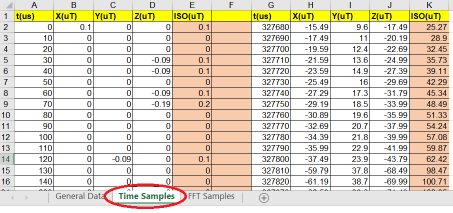
As an example, for the file shown in the following figure, the following should be set:
- Excel sheet: 2 (circled in red);
- Number of initial rows to skip: 1 (highlighted in yellow);
- Progressive number of columns to skip: 5,6,11 (highlighted in orange);
- Physical quantities: t, Bx, By, Bz (the field modulus is superfluous data);
- Unit of measurement: μs, μT, μT, μT;
- Separator between data: comma;
- Number of data column repetitions: 2.
There are 2 ways to perform the procedure:
- From the Chain from archive tab, specifying:
- Manufacturer of the measurement chain (optional, if indicated filters the chains)
- Measurement chain
- Measurement mode
- Chain settings
Selecting the Measurement mode populates the Conversion factor and Voltage offset, otherwise set by default to 1 and 0, respectively.
Selecting Chain Settings:- the File Structure tab is populated.
- a button is displayed that allows you to download the example text file corresponding to the chosen chain (2 buttons in the case of a calculation sheet: one for the file and a CSV corresponding to the sheet of interest), and a table with the values formatted according to the specific settings;
- Specifying the values needed to interpret the files in the
File Structure tab. Once this part of the procedure
is completed, import the data in JSON by clicking
on Import data in JSON (blue arrow pointing down).
This mode is priority: the parameters present in the JSON text area are considered in the processing, and if manually modified the original settings relating to the previously selected measurement chain are lost.
This sub-tab contains a text field and the buttons:- Import data in JSON (blue arrow pointing down) to import the parameters specified in the various fields in text format (according to the syntax of a JSON object);
- Export data from JSON (blue arrow pointing up) to fill the fields starting from a JSON object present in the appropriate text field;
In the User Files tab, one or more files containing the measurement data must be loaded, with a homogeneous structure also with regard to the units of measurement and compatible with what has been entered in the File Structure tab.
If the file loaded by the user is not compatible with what is specified in File Structure, unexpected results or an error message may be obtained from the test and processing programs.
The files must be loaded in the order in which they are produced by the instrumentation. Immediately after the selection they appear in alphabetical order, but the user can position them appropriately by dragging the name to the desired position.
Finally, by clicking on Send data the control procedures are performed on the data entered by the user, the files are uploaded to the server (the progress status is displayed in the appropriate scroll bar) and are stored in an appropriate format on the server side.
At the end:
- the 3 components of the induction in the time domain are present, and the data are passed to the actual processing part;
- the data are not compatible with the processing procedures, and are displayed in the space below in tabular and graphic format.
The allowed units are those given by the combination of a prefix corresponding to an exponent multiple of 3 and the unit of the physical quantities of interest (as per table).
For vector quantities (B, H, E, J, S) the values related to the projection along the axes are also allowed (Ex, Ey, Ez, Bx, ...).
| Grandezza | E | H | B | B | DELTAB | DELTAB | S | J | SAR | SA | U | DBDT | DBDT | V | I | t | f | W |
|---|---|---|---|---|---|---|---|---|---|---|---|---|---|---|---|---|---|---|
| $${\Unita\`}/{\Prefisso}$$ | V/m | A/m | T | G | T | G | W/m2 | A/m2 | W/kg | J/kg | J/m2 | T/s | G/s | V | A | s | Hz | W |
| y | yV/m | yA/m | yT | yG | yT | yG | yW/m2 | yA/m2 | yW/kg | yJ/kg | yJ/m2 | yT/s | yG/s | yV | yA | - | yHz | yW |
| z | zV/m | zA/m | zT | zG | zT | zG | zW/m2 | zA/m2 | zW/kg | zJ/kg | zJ/m2 | zT/s | zG/s | zV | zA | - | zHz | zW |
| a | aV/m | aA/m | aT | aG | aT | aG | aW/m2 | aA/m2 | aW/kg | aJ/kg | aJ/m2 | aT/s | aG/s | aV | aA | - | aHz | aW |
| f | fV/m | fA/m | fT | fG | fT | fG | fW/m2 | fA/m2 | fW/kg | fJ/kg | fJ/m2 | fT/s | fG/s | fV | fA | - | fHz | fW |
| p | pV/m | pA/m | pT | pG | pT | pG | pW/m2 | pA/m2 | pW/kg | pJ/kg | pJ/m2 | pT/s | pG/s | pV | pA | - | pHz | pW |
| n | nV/m | nA/m | nT | nG | nT | nG | nW/m2 | nA/m2 | nW/kg | nJ/kg | nJ/m2 | nT/s | nG/s | nV | nA | ns | nHz | nW |
| µ | µV/m | µA/m | µT | µG | µT | µG | µW/m2 | µA/m2 | µW/kg | µJ/kg | µJ/m2 | µT/s | µG/s | µV | µA | µs | µHz | µW |
| m | mV/m | mA/m | mT | mG | mT | mG | mW/m2 | mA/m2 | mW/kg | mJ/kg | mJ/m2 | mT/s | mG/s | mV | mA | ms | mHz | mW |
| V/m | A/m | T | G | T | G | W/m2 | A/m2 | W/kg | J/kg | J/m2 | T/s | G/s | V | A | s | Hz | W | |
| k | kV/m | kA/m | kT | kG | kT | kG | kW/m2 | kA/m2 | kW/kg | kJ/kg | kJ/m2 | kT/s | kG/s | kV | kA | - | kHz | kW |
| M | MV/m | MA/m | MT | MG | MT | MG | MW/m2 | MA/m2 | MW/kg | MJ/kg | MJ/m2 | MT/s | MG/s | MV | MA | - | MHz | MW |
| G | GV/m | GA/m | GT | GG | GT | GG | GW/m2 | GA/m2 | GW/kg | GJ/kg | GJ/m2 | GT/s | GG/s | GV | GA | - | GHz | GW |
| T | TV/m | TA/m | TT | TG | TT | TG | TW/m2 | TA/m2 | TW/kg | TJ/kg | TJ/m2 | TT/s | TG/s | TV | TA | - | THz | TW |
| P | PV/m | PA/m | PT | PG | PT | PG | PW/m2 | PA/m2 | PW/kg | PJ/kg | PJ/m2 | PT/s | PG/s | PV | PA | - | PHz | PW |
| E | EV/m | EA/m | ET | EG | ET | EG | EW/m2 | EA/m2 | EW/kg | EJ/kg | EJ/m2 | ET/s | EG/s | EV | EA | - | EHz | EW |
| Z | ZV/m | ZA/m | ZT | ZG | ZT | ZG | ZW/m2 | ZA/m2 | ZW/kg | ZJ/kg | ZJ/m2 | ZT/s | ZG/s | ZV | ZA | - | ZHz | ZW |
| Y | YV/m | YA/m | YT | YG | YT | YG | YW/m2 | YA/m2 | YW/kg | YJ/kg | YJ/m2 | YT/s | YG/s | YV | YA | - | YHz | YW |
Time data can be expressed in the following formats:
- numeric (in s, ms, μs or ns);
- hexadecimal (in 0.01 s), from whose conversion to decimal format we can go back to the first case;
- date/time, in which the possible representations of dates
and times are given in the following tables and the data is
represented as [DATE][T][TIME][Timezone]. The conversion to
numeric format is done through the function
strtotime; the decimal part is added later. For conventions used regarding time zones (MST, PDT, CEST...), see https://www.timeanddate.com/time/zones/.
For example, the following values are equivalent:
- 19901028192030Z
- 19901028 192030Z
- 19901028T192030Z
- 1990-10-28T19:20:30Z
- Wed 1990-10-28T19:20:30Z (the name of the day of the week is neglected)
- 19901028192030+7
- 19901028192030+07
- 19901028192030+0700
- 19901028 192030+0700
- 19901028T192030+0700
- 1990-10-28T19:20:30+07:00
- 1990-10-28T19:20:30GMT+07:00
- strtotime("1970/01/01 00:00:00") = -3600
- strtotime("1970/01/01 00:00:00Z") = 0 (1 hour difference for time zone)
- strtotime("00:00:00") = 1532642400 (implies today's date)
- strtotime("00:00:00Z") = 1532649600 (2 hours difference, one for daylight saving time and one for the time zone)
| Date related formats | |
|---|---|
| General form | Example |
| dd-mmm-yy | 28-OCT-90 |
| dd-mmm-yyyy | 28-OCT-1990 |
| mm/dd/yy | 10/28/90 |
| mm/dd/yyyy | 10/28/1990 |
| dd.mm.yy | 28.10.90 |
| dd.mm.yyyy | 28.10.1990 |
| yyyyddd | 1990301 |
| yyyy.ddd | 1990.301 |
| yyyy/mm/dd | 1990/10/28 |
| yyyymmdd | 19901028 |
| mmm yyyy | OCT 1990 |
| Nome del mese | OCT |
| yyyy-mm-dd | 1990-10-28 |
| yy-mm-dd | 90-10-28 |
| yyyy.mm.dd | 2015.03.17 |
| yy.mm.dd | 15.03.17 |
| mmm/dd/yyyy | Mar/16/2006 |
| mmm/dd/yy | Mar/16/06 |
| mm/dd/yy | 2/1/6 |
| Time related formats | |
|---|---|
| General form | Example |
| hh:mm | 01:42 |
| hh:mm:ss | 01:42:37 |
| hh:mm:ss.s | 01:42:37.3657454 |
| hh:mm:ss [AM] | 07:20:30 AM |
| hh:mm:ss [PM] | 07:20:30 PM |
| hhmmss | 192030 |
| hhmmss.s | 192030.2454 |
| TZD (TimeZone Designator) related formats | |
| +|-hh:mm | +01:00 |
| +|-hhmm | +0100 |
| +|-hh | +01 |
| +|-hh | +1 |
| Z | Z |
| ... | MST (PDT, CEST...) |
Selecting a chain operating in the frequency domain, if the measured quantity is one of:
- Electric Field
- Magnetic Flux Density
- Voltage
- Current
- Power
data can be compared with a homogeneous limit among those present in the documents:
- MSFC-SPEC-521: Electromagnetic compatibility requirements for equipment and susbsytems
- MIL-STD-461E: Requirements for the control of electromagnetic interference characteristics of subsystems and equipment
- ECSS-E-ST-20-07C: Space engineering - Electromagnetic compatibility
The measured quantity must be expressed in one of the units of measurement of the International System, not in dB. The appropriate conversions are carried out before the results are displayed.
Once the limit of interest has been selected, the frequency extremes are displayed in the fields:
- Minimum frequency
- Maximum frequency
These values can be edited to narrow the range displayed in the output graph.
If it is necessary to use an upper limit of a constant value to the selected reference, the difference (expressed in dB) must be reported in the Modify limit field.
If the measured quantity represents a voltage, 2 additional boxes appear, in which to insert any corrections due to:
- Antenna factor: is activated by selecting Enable correction with antenna factor. The relevant data, expressed in Hz and dB/m, must be copied from 2 columns of a spreadsheet. The menu with the limits is automatically updated with the limits for the electric field. By deselecting the option, the voltage limits reappear.
- LISN: is activated by selecting Enable correction for LISN. The relevant data, expressed in Hz and dBµV, must be copied from 2 columns of a spreadsheet. The option is disabled if the correction for antenna factor is enabled.
By pressing Compare, a graph is created in which the trends of the selected limit and the data contained in the loaded file are reported. The warning window may appear for:
- No measurement result falls within the frequency interval of the selected limit: in this case, only the trend of the limit is represented in the graph.
- Total exceedances: # (number of exceedances)
Download the exceeding.txt file: by clicking on exceeding.txt you download a text file locally that displays in 3 columns:- the frequency at which the limit is exceeded
- the measured value, possibly obtained by linear interpolation between the measurements at a frequency lower and higher than the one considered
- the limit calculated at that frequency value
- Total NON-exceedances: # (number of non-exceedances)
Download the non-exceeding.txt file: as above
Keywords: Processing of data files, Time domain, Frequency domain, Measurement chains