The Weighted Peak Method - Examples and Critical Issues

Action Values of Legislative Decree 159/2016 integrated with the reference levels ICNIRP-2014

See also the specifications of the filters for the calculation of the weighted peak indices in the frequency domain, referred to the lower (sensory effects) and upper (health effects) VA of Legislative Decree 159/2016.

Please note:

all the WP indices cited refer to reference values and action levels relating to the prevention of sensory effects.
The red values are clearly incorrect values, originating from the various critical issues that we want to present and discuss in the document; black values are exact or reasonably correct.

LEGEND

IWP-FD-PWL: Weighted peak index calculated in the frequency domain with reference to the exact (piecewise linear) weighting curves
IWP-FD-RCF: Weighted peak index calculated in the frequency domain with reference to the weighting curves approximated with analogue resistance and capacitance filters
IWP-TD: Weighted peak index calculated in the time domain

Examples based on waveforms from real measurements

Transcranial Magnetic Stimulation

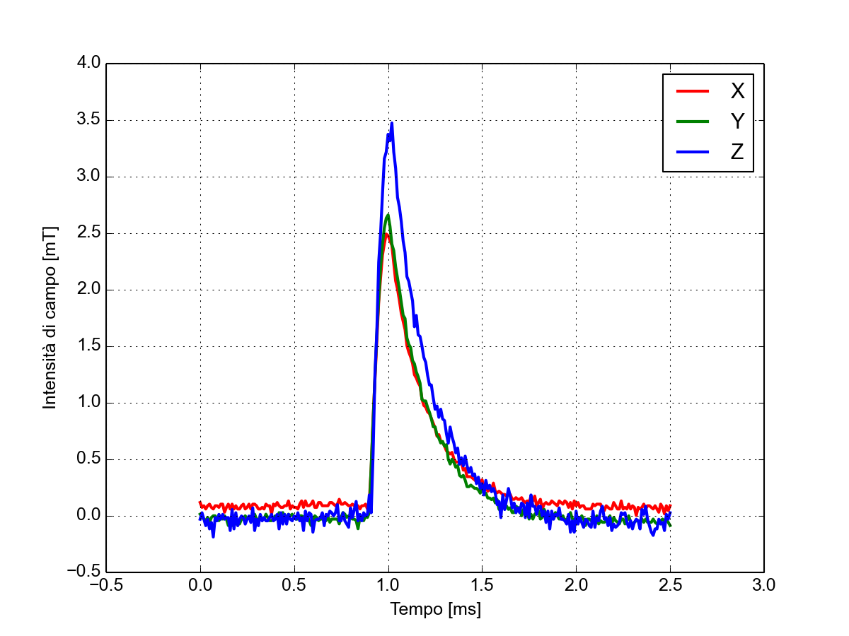
Notes	Measurement at 32 cm from an HP 9784-00 applicator connected to a Magstim 200 stimulator with 100% power.
Magnetic field waveform
Peak indices weighted	IWP-FD-PWL = 15.5 IWP-FD-RCF = 17.3 IWP-TD = 17.5

Remarks

This is a single-event signal of limited duration, generated by the discharge of a monophasic transcranial magnetic stimulation pulse. We observe an excellent correspondence between the TD and FD-RCF indices and a modest discrepancy between these and the FD-PWL index, probably due to the differences between the respective weight functions.

Gradient fields in magnetic resonance imaging

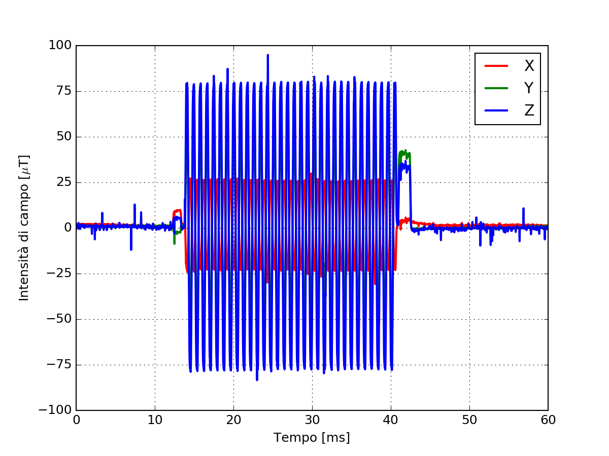
Notes	Measurement acquired at the mouth of the bore of a 1.5 T Philips Achieva Nova tomograph (Fatebenefratelli Hospital, Rome), using an Axial EPI sequence segment with 21 0.5 mm slices.
Magnetic field waveform
Weighted peak indices	IWP-FD-PWL = 0.310 IWP-FD-RCF = 0.326 IWP-TD = 0.327

Remarks

Fragment (a single burst extracted from a sequential repetition) of the signal produced by the measurement of gradient fields generated by a magnetic resonance apparatus. An excellent correspondence is observed between the TD and FD-RCF indices and a modest discrepancy between these and the FD-PWL index, probably due to the differences between the respective weight functions.

Examples based on ad hoc

waveforms

1) Periodic waveform

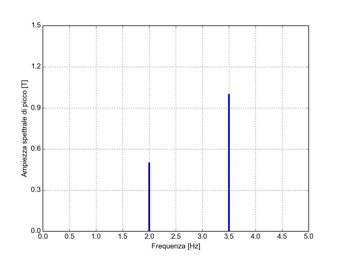
Mathematical expression: sum of a sinusoid with frequency 2 Hz and amplitude 0.5 T and a cosine with frequency 3.5 Hz and amplitude 1 T; the overall period of the waveform is 2 s.
Spectrum with observation time of 8 s; this observation time is a multiple of the period of the waveform (it includes 16 cycles of the lower frequency component and 28 cycles of the higher frequency component) and therefore does not give rise to spectral leakage.
Weighted Peak Indices	IWP-FD-PWL = 50.2 IWP-FD-RCF = 47.0 IWP-TD = 47.2
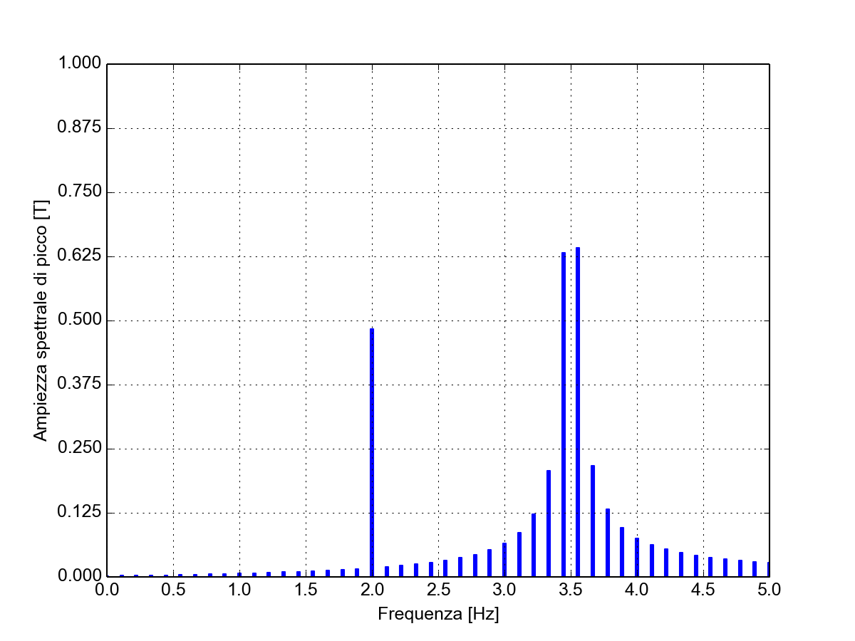
Spectrum with observation time of 9 s; this observation time is NOT a multiple of the waveform period (it includes 18 cycles of the lowest frequency component and 31.5 cycles of the highest frequency component) and therefore gives rise to spectral leakage on the second line. To be precise, this is long range spectral leakage with associated (modest) spectral interference on the first line.
Weighted Peak Indices	IWP-FD-PWL = 639 IWP-FD-RCF = 561 IWP-TD = 47.2
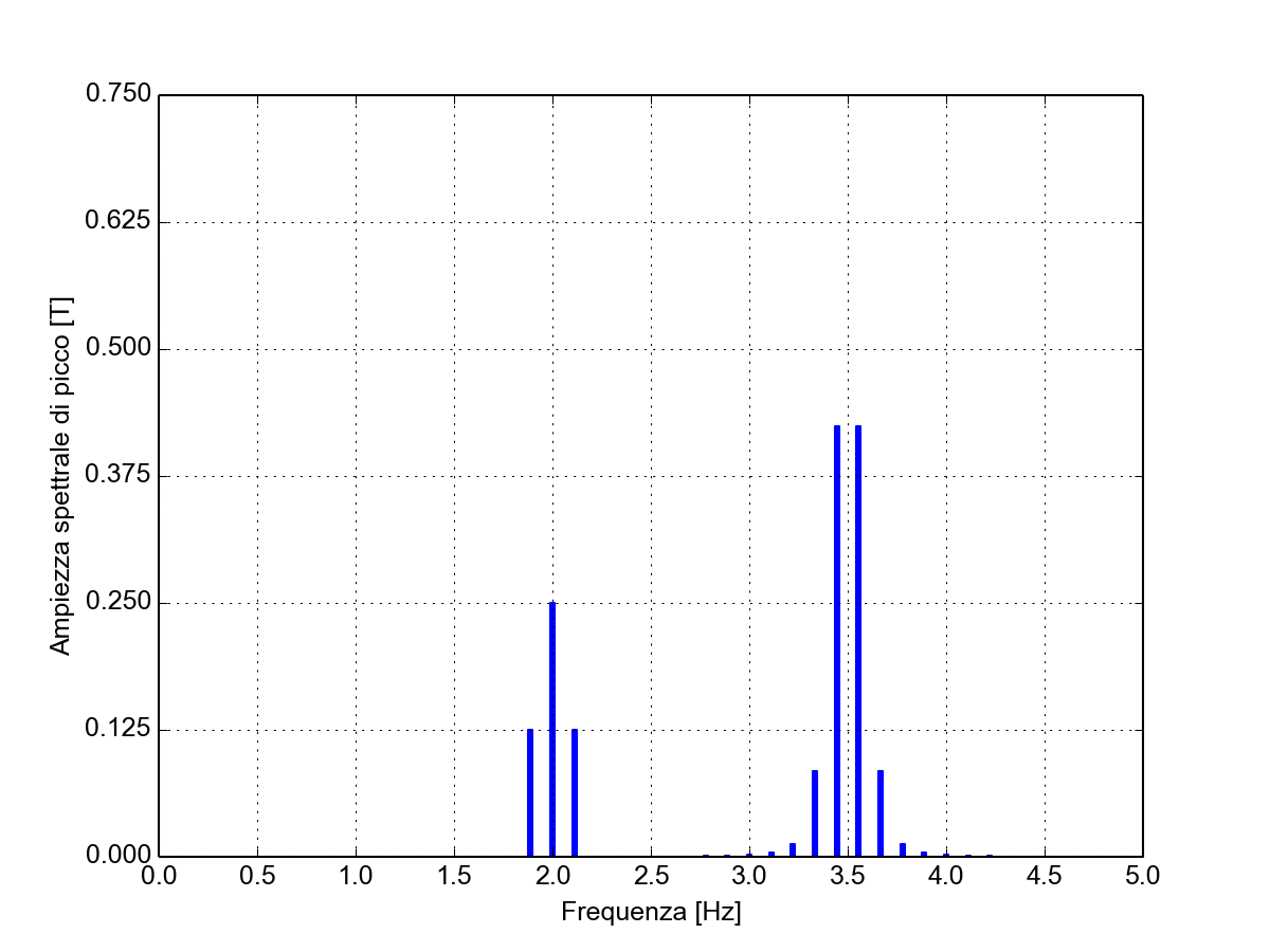
Spectrum with observation time of 9 s after Hann windowing; the windowing has the purpose of transforming the long range spectral leakage into short range spectral leakage, also removing the spectral interference between the two lines.
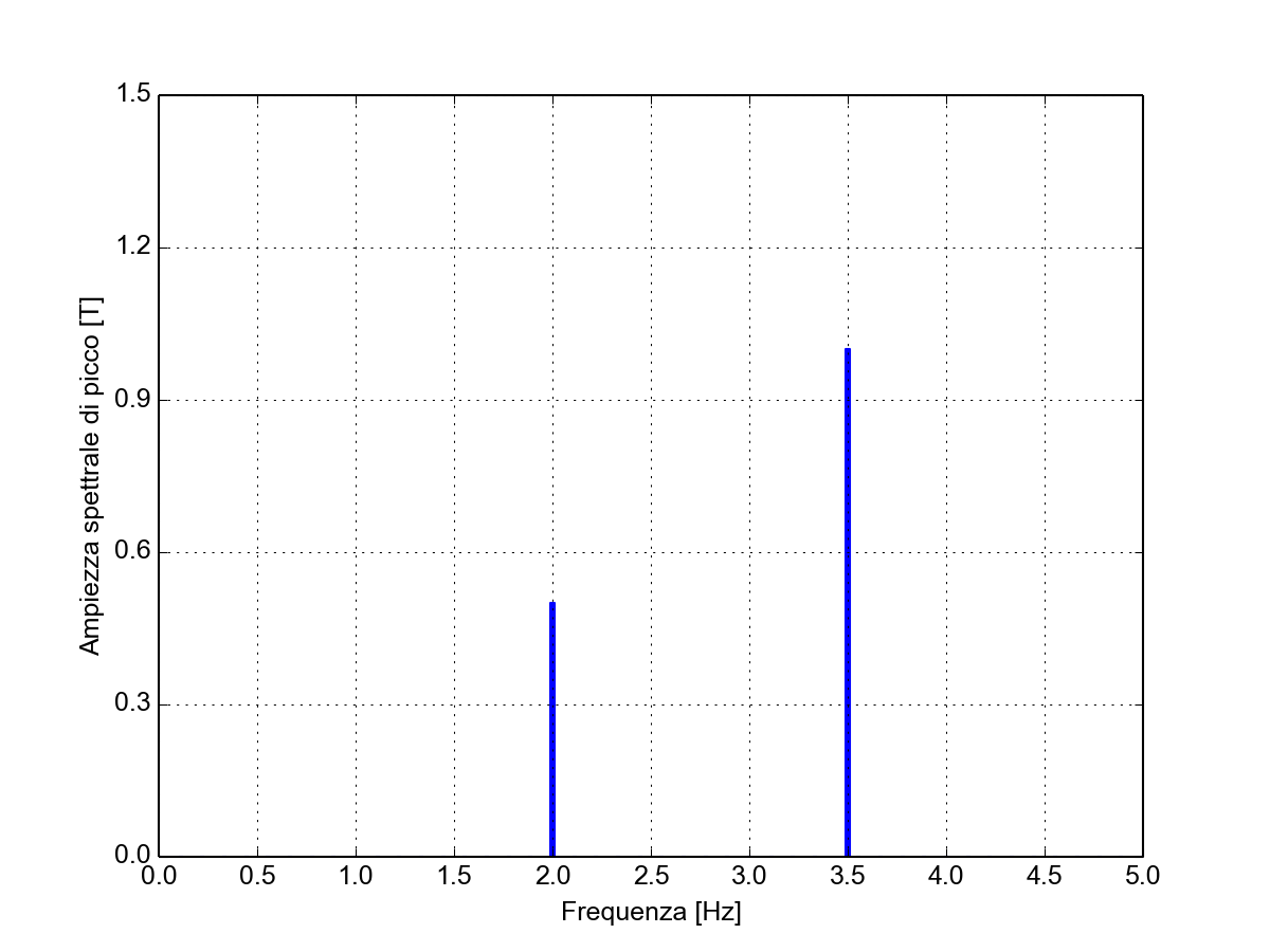
Spectrum with 9 s observation time after Hann windowing and spectral interpolation: the spectral leakage has been completely removed.
Weighted Peak Indices	IWP-FD-PWL = 50.4 IWP-FD-RCF = 47.4 IWP-TD = N/A

Observations

With this example, in addition to documenting the spectral leakage, its effect on the Weighted Peak Indices, interference and spectral interpolation, it is shown that the leakage can affect even just one line of the spectrum. We chose to make it appear on the second line (the one with the highest frequency), in order to maximize its consequences on the WP indices. We used a cosine for this line and a truncation of half a period (or better of 1 s equal to 3.5 periods), in order to maximize the difference between the beginning and the end of the signal and therefore the leakage.

2) Double step

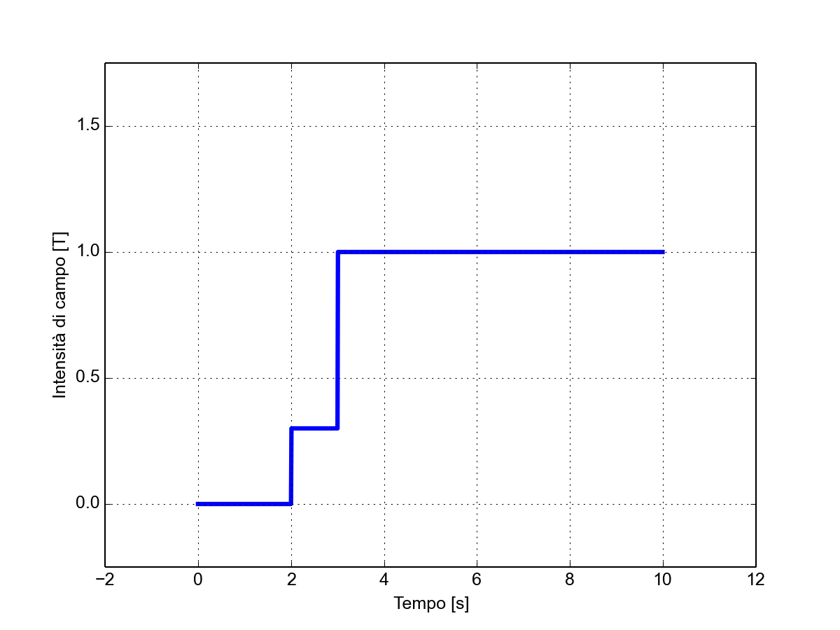
Square waveform, initially at zero value, which presents a first step of +0.3 T at t = 2 s and a further step of +0.7 T at t = 3 s, to then remain indefinitely at the value of 1 T.
Magnetic field waveform
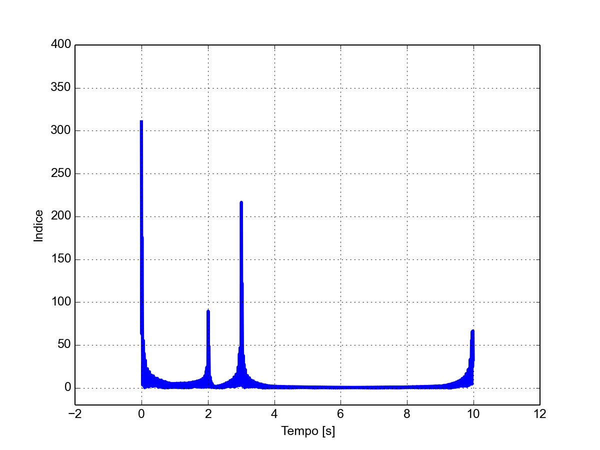
FD-PWL index
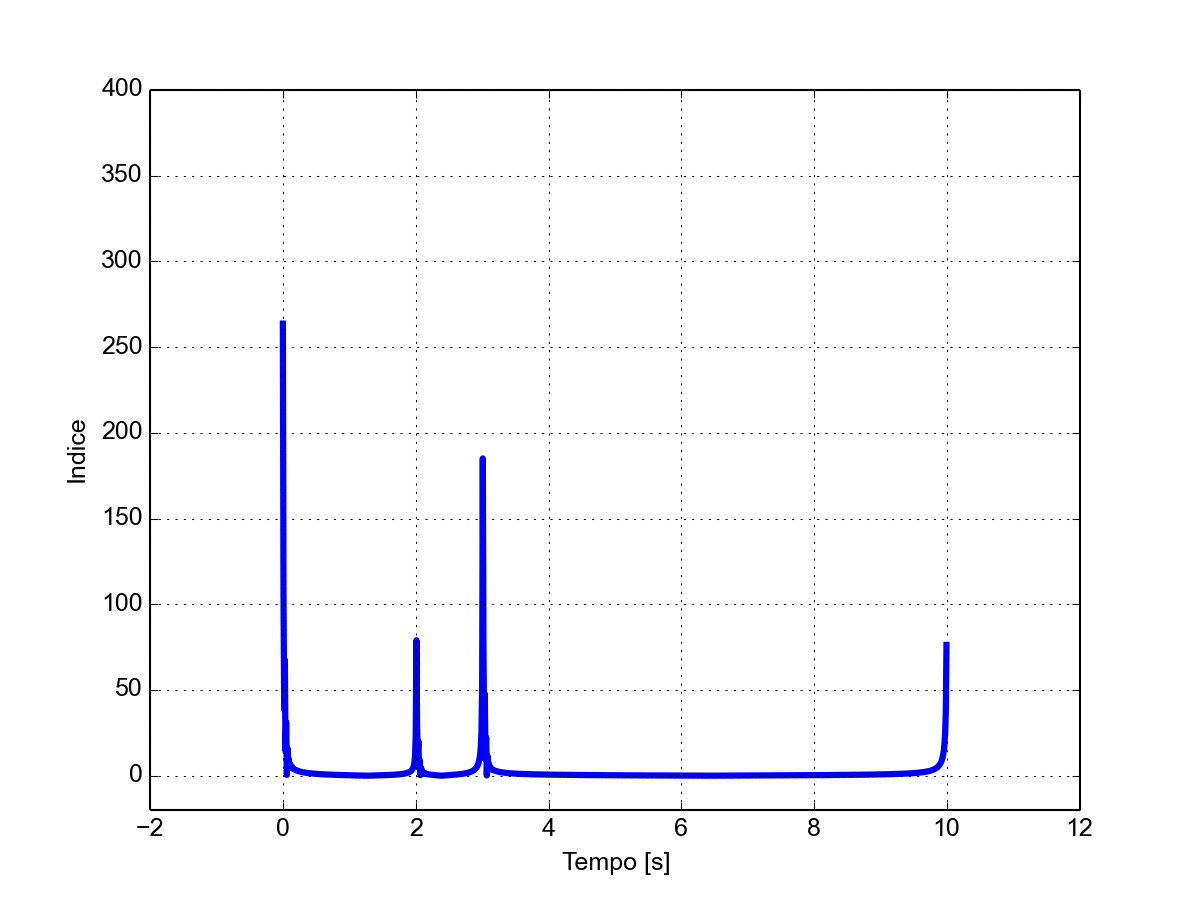
FD-RCF index
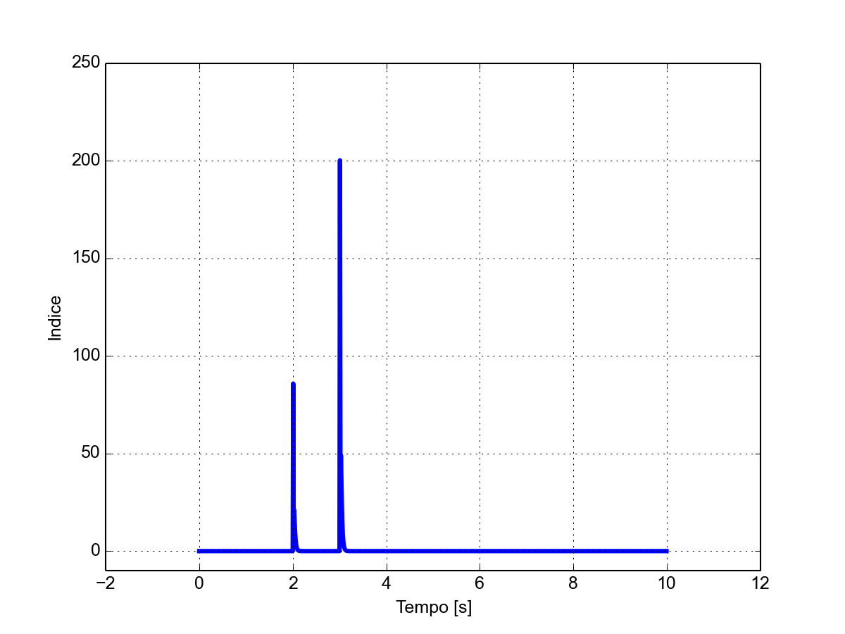
TD index
Weighted Peak Indices	IWP-FD-PWL = 310 IWP-FD-RCF = 264 IWP-TD = 200
Weighted Peak Indices between 1 s and 9 s	IWP-FD-PWL = 217 IWP-FD-RCF = 185 IWP-TD = 200

Observations

Due to the limited observation time and the periodicity imposed by the DFT, in the evaluation of the index in FD mode, in addition to the two peaks corresponding to the two steps actually present, a further peak appears corresponding to the fictitious variation of the field intensity from +1 T to 0 T that occurs at the end of the observed interval. This index peak, absent in the TD evaluation, is predominant, because the fictitious step from which it originates has a greater amplitude than the two steps actually present (in absolute value it is equal to their sum). In some cases, it is possible to determine a correct index also by operating in the frequency domain, ignoring a congruent number of samples at the beginning and at the end of the FD index waveform as a function of time.

3a) Initial artifact (absent)

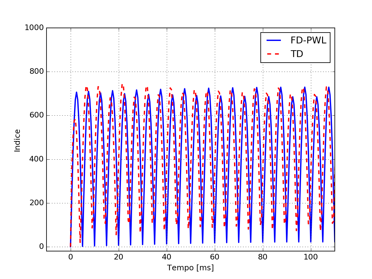
Mathematical expression: sum of two sinusoids of unit amplitude, in phase with each other, one at 2.5 Hz and the other at 100 Hz. Period 0.4 s. Observation time 4 s (no spectral leakage).
Waveform of the WP index calculated in FD-PWL and TD modes
Weighted Peak Indices	IWP-FD-PWL = 729 IWP-FD-RCF = 742 IWP-TD = 734

Observations

The example highlights the criticality of the TD approach when dealing with a signal that at the beginning of the observation has a value very different from zero. As can be seen in this first sub-example, the phenomenon does not occur with the sum of sinusoids (since the signal in this case starts from zero). The phenomenon does not occur in any case in the frequency domain (FD).

3b) Initial artifact (present)

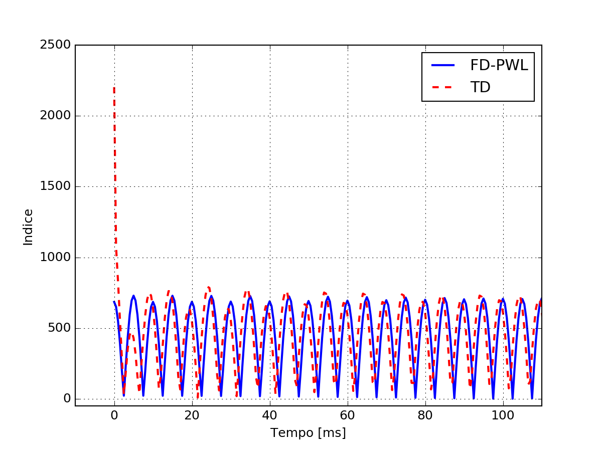
Mathematical expression: sum of two cosine waves of unit amplitude, in phase with each other, one at 2.5 Hz and the other at 100 Hz. Period 0.4 s. Observation time 4 s (no spectral leakage).
Waveform of the WP index calculated in FD-PWL and TD modes
Weighted Peak Indices	IWP-FD-PWL = 729 IWP-FD-RCF = 742 IWP-TD = 2203 (initial) IWP-TD = 734 (after the transient)

Observations

The example highlights the criticality of the TD approach when dealing with a signal that at the beginning of the observation has a value very different from zero. In this second sub-example we see how, due to the abrupt start, an intense initial artifact appears in the WP index calculated in the time domain, which must be ignored to acquire the correct WPI value. The phenomenon does not occur in any case in the frequency domain (FD).

4a) Cosine burst

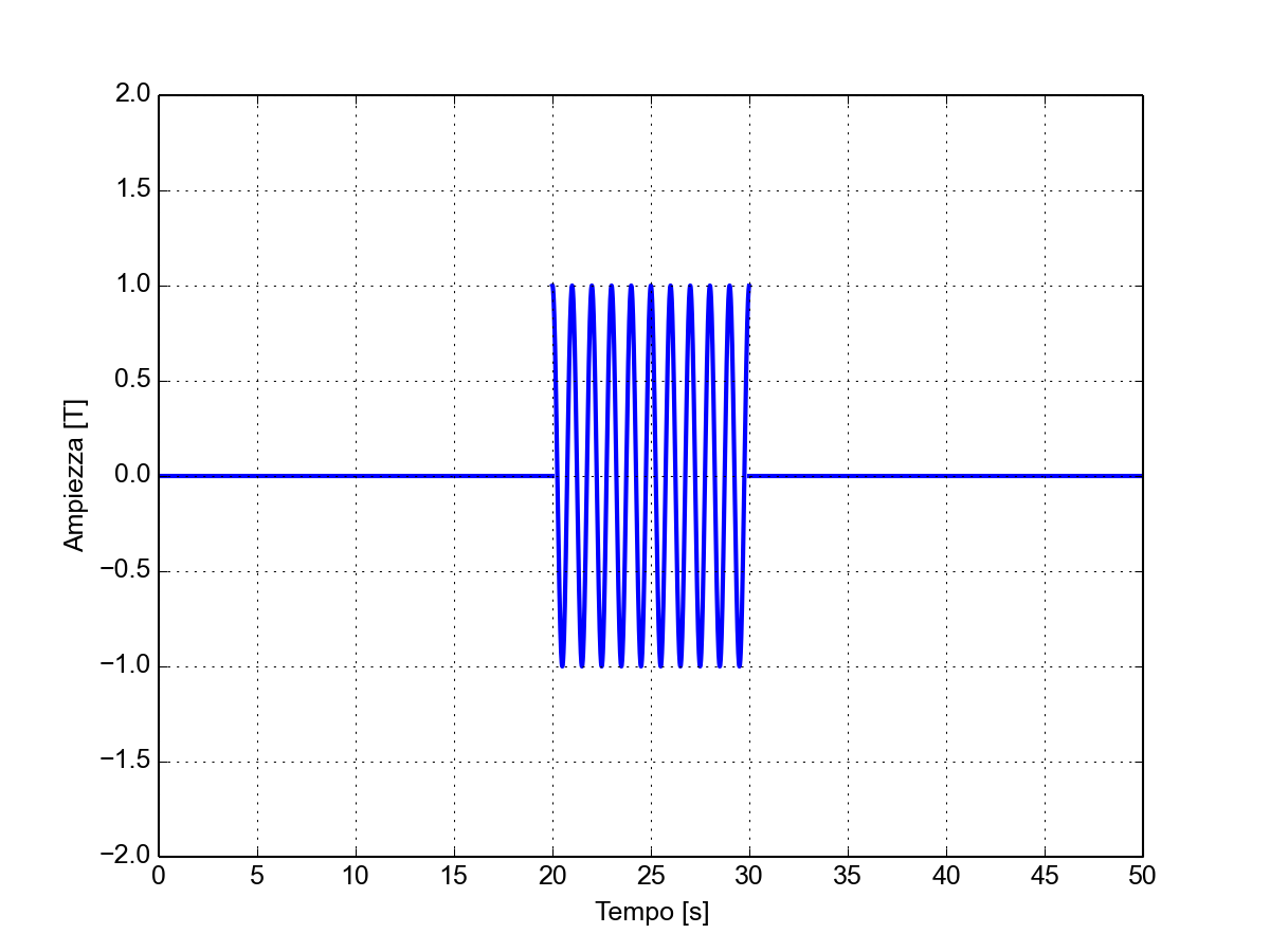
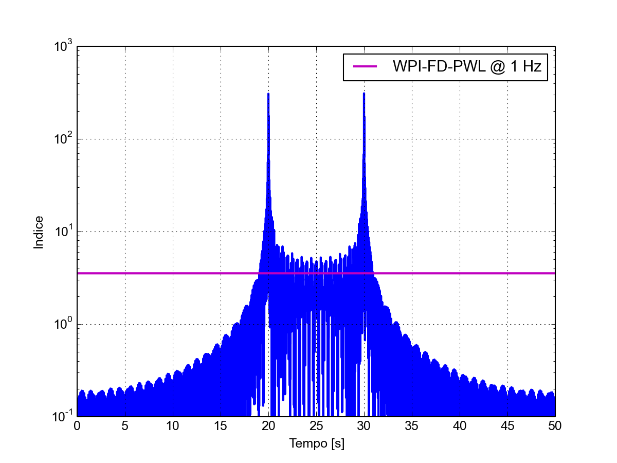
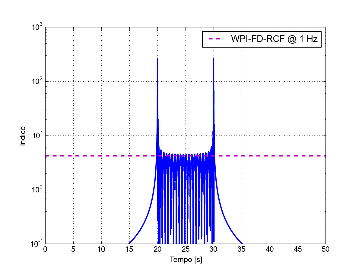
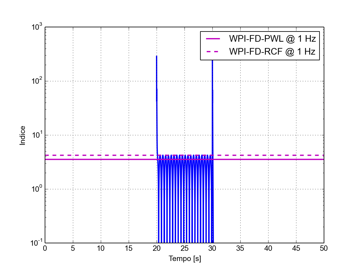
Cosine burst: initially at zero value for 20 s, followed by a cosine wave at 1 Hz with peak amplitude 1 T and duration 10 s, followed by a stretch at zero value for another 20 s.
Signal waveform
Waveform of WP index calculated in FD-PWL mode
Waveform of WP index calculated in FD-RCF mode
Waveform of WP index calculated in TD mode
Weighted Peak Indices	IWP-FD-PWL = 311 IWP-FD-RCF = 267 IWP-TD = 289

Observations

Unlike case 3), in this example the initial transient is not an unwanted artefact (to be avoided or corrected, because it originates from the way the observation starts), but rather a characteristic of the observed signal. When, as in this sub-example, this signal is a cosine, the transition is more abrupt (the field is discontinuous at the beginning of the burst) and generates very high indices.

4b) Sine burst

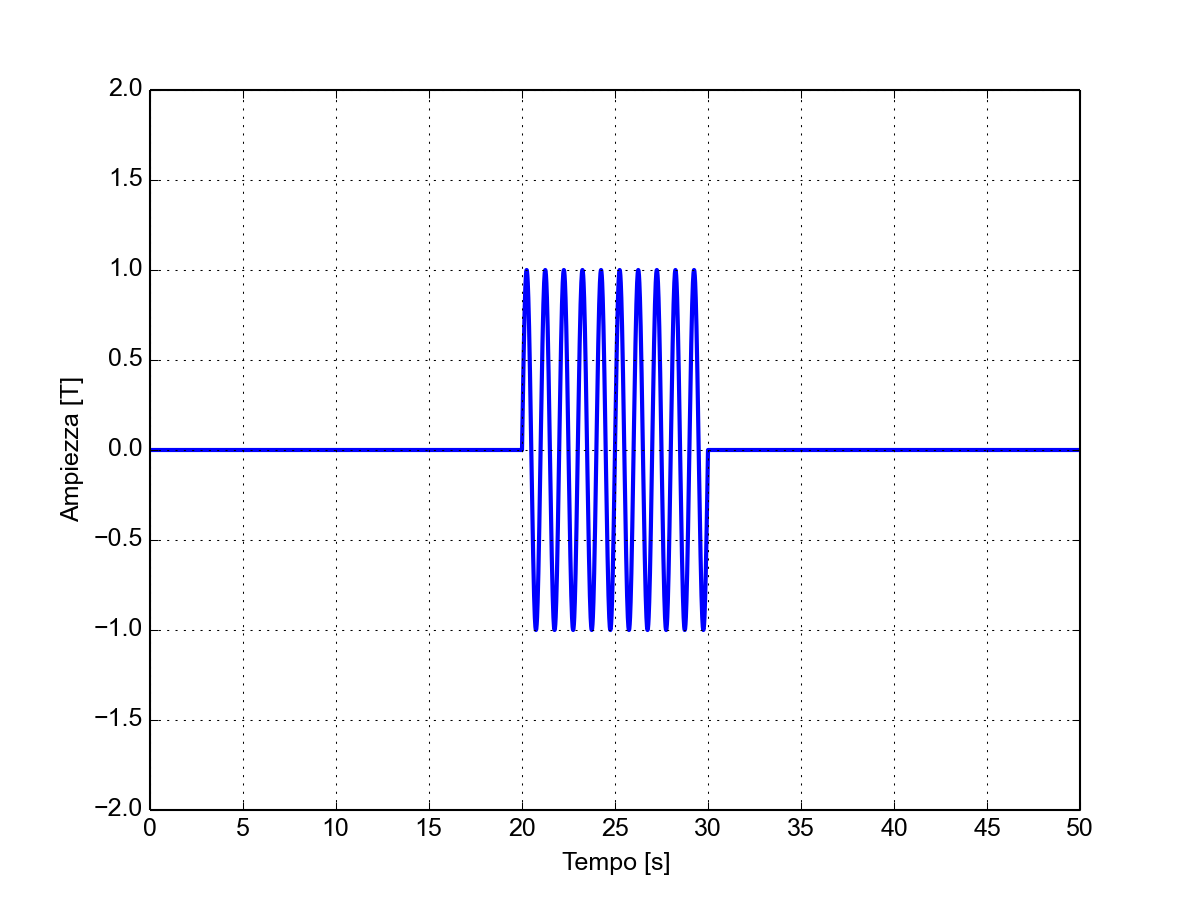
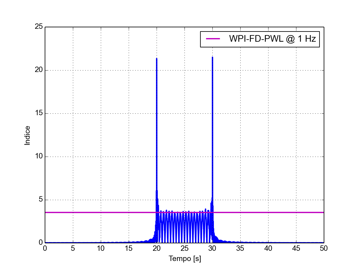
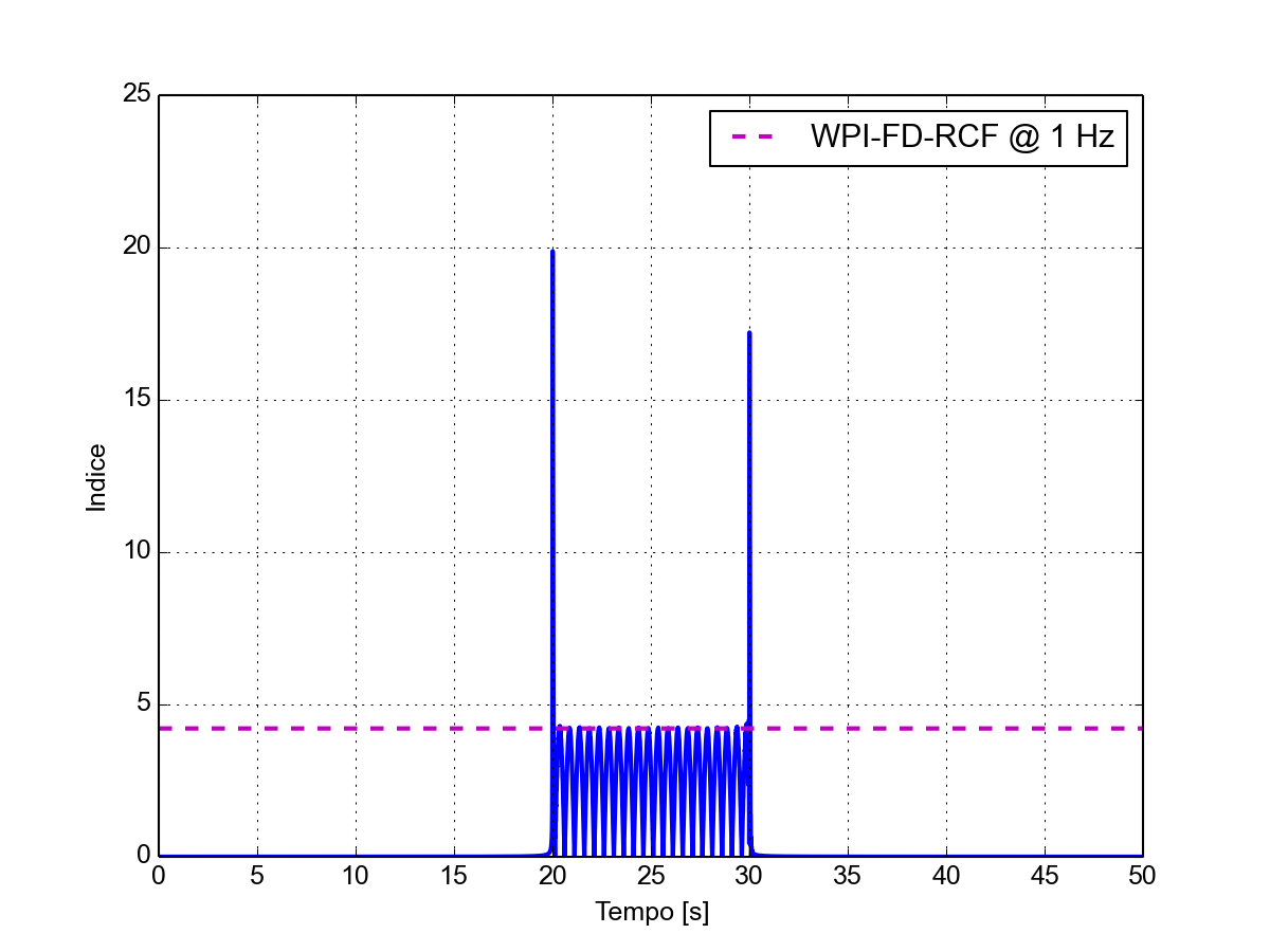
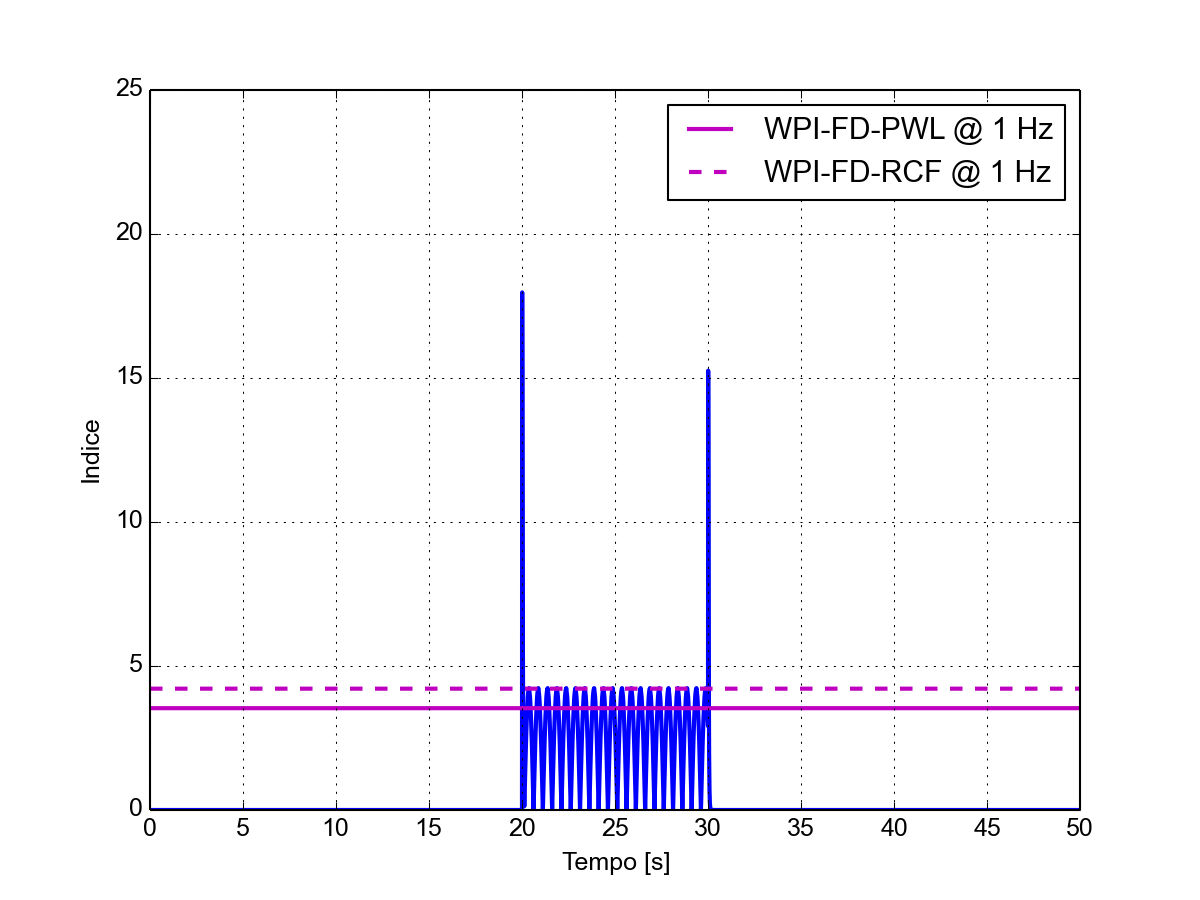
Sine burst: initially at zero value for 20 s, followed by a 1 Hz sinusoid with peak amplitude 1 T and duration 10 s, followed by a stretch at zero value for another 20 s.
Signal waveform
Waveform of WP index calculated in FD-PWL mode
Waveform of WP index calculated in FD-RCF mode
Waveform of WP index calculated in TD mode
Weighted Peak Indices	IWP-FD-PWL = 21.5 IWP-FD-RCF = 19.9 IWP-TD = 18.0

Observations

Unlike case 3), in this example the initial transient is not an unwanted artifact (to be avoided or corrected, because it originates from the way the observation starts), but rather a characteristic of the observed signal. When, as in this sub-example, this signal is a sine, the discontinuity at the beginning of the burst does not concern the value of the field, but only its derivative, and therefore the indices are lower than in the previous case, but still much higher than the value that would be the sinusoid.

4c) Raised cosine burst

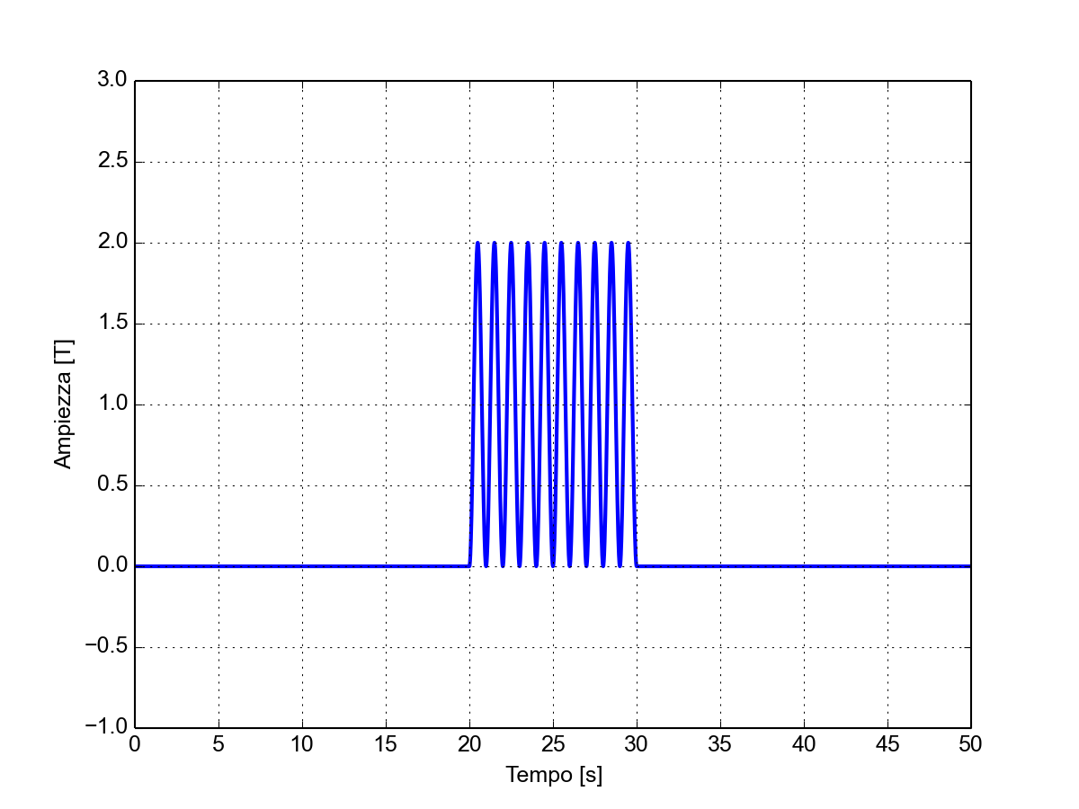
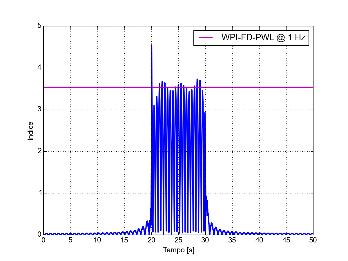
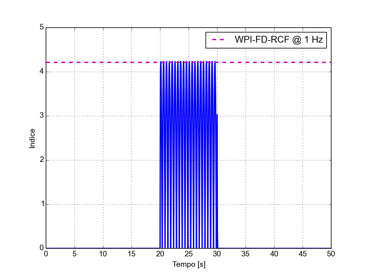
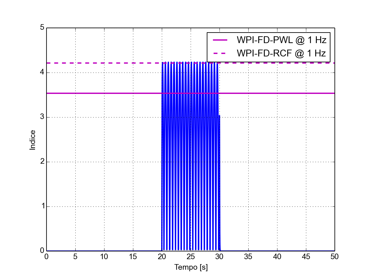
Raised cosine burst: initially at zero value for 20 s, followed by a raised cosine with offset 1 T, peak amplitude 1 T, frequency 1 Hz and duration 10 s, followed by a stretch at zero value for another 20 s.
Signal waveform
Waveform of WP index calculated in FD-PWL mode
Waveform of WP index calculated in FD-RCF mode
Waveform of WP index calculated in TD mode
Weighted Peak Indices	IWP-FD-PWL = 4.5 IWP-FD-RCF = 4.2 IWP-TD = 4.2

Observations

Unlike case 3), in this example the initial transient is not an unwanted artifact (to be avoided or corrected, because it originates from the way in which the observation begins), but rather a characteristic of the observed signal. When, as in this sub-example, this signal is a raised cosine, designed so that both the field and its derivative are continuous at the beginning of the burst, the values of the indices are perfectly aligned with those of the sinusoid.

Keywords: Weighted Peak