Ideal screen
Purpose
The sizing of a shield is a laborious process, which involves several phases and often begins with the choice of the sheet of material to work with. This application allows you to evaluate (and therefore size) the shielding effectiveness of a plate taking into account the following factors:
- the frequency of the field;
- the nature of the source (whether an electric or magnetic field);
- the distance between the source and the plate (and therefore the condition whether this is hit by a plane wave or is instead exposed to a reactive field);
- the physical characteristics of the plate and the material it is made of (thickness, electrical conductivity and magnetic permeability).
The application uses a calculation model well-established in the literature and summarised below, in which the plate is assimilated to an ideal screen (i.e. flat, infinitely extended, homogeneous and of constant thickness). In this model, the shielding effectiveness is expressed as the sum of four terms: the reflection on the first and on the second discontinuity surface of the plate, the absorption inside the latter and the effect of multiple reflections (i.e. the rebounds between the two surfaces).
Shielding effectiveness
The shielding effectiveness (SE, Shielding Effectiveness) quantitatively expresses the ability of a screen to reduce the intensity of the electromagnetic signal in a given region.
The shielding effectiveness with respect to the electric field is defined by:
ove:
- E1 expresses the amplitude of the electric field at a point in the region of interest before the shield is positioned;
- E2 expresses the amplitude of the electric field at the same point, after the shield is positioned.
Similarly, the shielding effectiveness against the magnetic field is defined as:
Electromagnetic field as a function of distance from the source
- Reactive field zone (or induction zone): in the vicinity of the source, the electric and magnetic fields must be determined independently and the coupling with material objects must be evaluated separately. The ratio between the amplitudes of the electric field and the magnetic field (field impedance) depends on the technical characteristics of the source.
- Radiative field zone: for distances from the source greater than the wavelength, the field has lost direct links with the source, the electric and magnetic components are linked to each other. The fields of radiative origin become significant (determined by the mutual generation between the electric and magnetic fields): the electromagnetic field is formed, of which the electromagnetic wave is a form of propagation. The field impedance depends solely on the characteristics in which the medium propagates:
In vacuum:
ove:
- ε0: dielectric constant (8,854 pF/m);
- μ0: absolute magnetic permeability (0,4π μH/m).
The ideal screen
By ideal screen we mean a homogeneous flat plate indefinite and of uniform thickness.
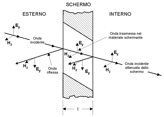
The wave is partly reflected, partly transmitted. The loss of power associated with the first reflection is indicated by RdB(1) (≥ 0).
The wave transmitted in the shielding material undergoes an attenuation due to the dissipation of energy by the Joule effect, AdB (≥ 0).
On the second interface the wave undergoes a second reflection and a consequent attenuation RdB(2) (≥ 0).
Contribution to the shielding effectiveness due to multiple reflections: BdB (≤ 0).
The shielding effectiveness depends on the contribution of these 4 phenomena:
From the continuity of the tangential components of the fields we have that:
and from the definition of field impedance:
Assuming that the wave impedance in the first material is the same on both sides of the screen and that the reflections on both surfaces can be described as a transition between two undefined homogeneous half-spaces, for the electric field on the first interface we find:
Similarly on the second interface:
Per il campo magnetico sulla prima interfaccia:
Similarly on the second interface:
Si ricava:
and it is formally equal for electric and magnetic fields.
Determination of ζ1
Depending on whether the sources are electric or magnetic fields, the impedance has a different trend:
| Distance from the source r | Electric field sources |
|---|---|
| Wave impedance in air or vacuum, as a function of the distance from an electrical source (internal impedance ζS > ζ0) | |
| Distance from the source r | Magnetic field sources |
|---|---|
| Wave impedance in air or vacuum, as a function of the distance from a magnetic source (internal impedance ζS < ζ0) | |
|
|
|
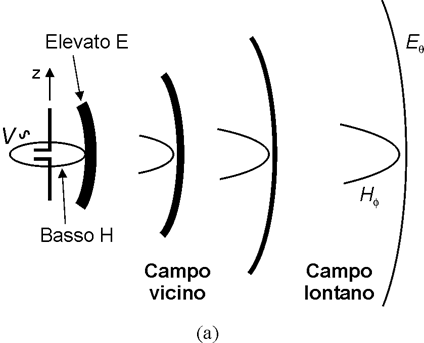
For an elementary electric dipole (consisting of a straight conductor, thin and short if compared with λ, supplied with a uniform current distribution) from the solution of Maxwell's equations in the frequency domain we obtain the equations for the fields: |
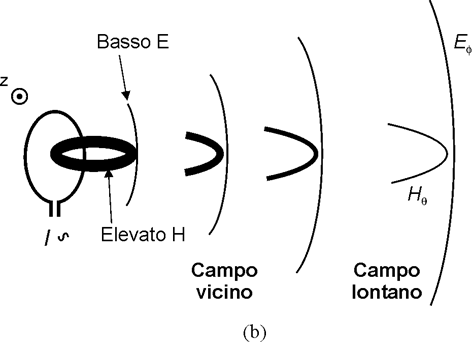
For a small coil (in terms of wavelength, i.e. 2πr ≪ λ) supplied with a sinusoidal current at frequency f uniformly distributed on it, the solution of Maxwell's equations leads to: |
Approximating an electric field source with an elementary electric dipole (on the left) and a magnetic field source with a coil (on the right), both of which are small in size compared to the wavelength, from Maxwell's equations we can obtain the trend of the electric and magnetic field and therefore of the impedance as illustrated in the following graph:
a partire da:
For k we can distinguish the cases:
- k ≃ λ/{2πr} for a high impedance source and r ≤ λ/2π;
- k ≃ {2πr}/λ for a low impedance source and r ≤ λ/2π;
- k ≃ 1 for any type of source and r ≥ λ/2π.
Determination of ζ2 and AdB
The depth of penetration into a conductor (distance over which the current density decreases by e times compared to the surface current density):
in the case of good conductors ( ) it simplifies:
where:
- f: wave frequency;
- σ: material conductivity;
- μ: magnetic permeability.
Contribution to shielding effectiveness due to absorption in the metal:
Barrier impedance ζ2 of a flat screen, as a function of its thickness t and the electromagnetic characteristics of the material it is made of:
Degradation of shielding effectiveness due to multiple reflections
The contributions due to multiple reflections have undergone – with respect to the main contribution – at least two more crossings of the screen, with consequent attenuations due to absorption in the same. It can be demonstrated that:
Magnetic classification of materials
Based on the value of the relative magnetic permeability, materials are classified into:
- paramagnetic materials, if μr ≳ 1 (e.g.: air, aluminum, tungsten);
- diamagnetic materials, if μr < 1 (e.g.: gold, copper);
- ferromagnetic materials, if μr ≫ 1 (e.g.: iron, nickel, cobalt).
In this last case, it is assumed that μr follows the Cole-Cole relaxation function:
where:
- f1/2: the frequency value for which the permeability takes on an intermediate value between the low and high frequency ones (set μ∞=1);
- α: the parameter that specifies how fast the relaxation occurs.
The following graph shows the trend of the real part of the permeability for different values of α, with f1/2 = 100 kHz and μr = 11000.
Internal documentation
You can access the document Riduzione e contenimento dell'esposizione, calcoli previsionali e schermature present on this portal.
Bibliographic references
- J.D.Kraus: Electromagnetics, McGraw-Hill International Student Edition, Singapore 1984.
- CEI (Comitato Elettrotecnico Italiano): Guida ai metodi di calcolo dei campi elettrici emagnetici generati da linee elettriche, Norma CEI 211-4, Milano, 1996.
- D.Andreuccetti: Manuale del programma CAMPI per il calcolo del campo elettrico e dell'induzione magnetica generati da linee elettriche versione 4.1, CNR - Istituto di Fisica Applicata Nello Carrara, Firenze, maggio 2002.
- AA.VV.: La schermatura dei campi elettrici, magnetici ed elettromagnetici: principi generali, aspetti teorici e applicazioni pratiche, Franco Angeli Editore Milano 2006, a curadi Paolo Bevitori.
- White D.R.J.: A handbook on electromagnetic shielding materials and performance, Don White Consultants Inc., Germantown (USA) 1975.
- White D.R.J.: Shielding design. Methodology and procedures, Interference Control Technologies, Gainesville (USA) 2006.
3D visualization of the attenuation
The scene shows the source (red sphere) → shield → receiver (green sphere) system. The coloured plane is the real part of the field travelling towards the shield: on the source side a standing wave builds up because almost all the field is reflected (term R); inside the shield the field decays by absorption (term A); beyond the shield only the attenuated transmitted fraction arrives (−SE dB). The arrows show the power flow. The red source can be dragged: it changes the distance r from the shield, and with it the wave impedance Z1(f, r) of the model, so the SE is seen to move from the near to the far field (r and kr are shown next to the source). The Source selector switches between magnetic and electric dipole, which in this model have different asymptotes. The labels in the scene carry the values of the model (SE, R, A, B, |Γ|, τ, δ). Rotate and zoom with the mouse; drag the probe to read the local field level.
Note: the numbers are those of the ideal shield model of this page, with real impedances and near/far-field asymptotes, not the real-conductor ones of the other applications. The geometry of the scene is qualitative: the representation wavelength is fixed and the thickness is enlarged. Material and thickness are taken from the Data input tab; press «Update» after changing them.
The controls above the scene:
- Frequency: the slider spans the whole range of the model;
- Source: plane wave, magnetic dipole or electric dipole;
- Thickness: acts on the scene alone and leaves the value in the data tab untouched;
- Comparison between the first two materials: splits the scene in half, one material each;
- Mode: switches between the wave and the amplitude view;
- Update from entered data: to be pressed after changing material or parameters in the Data Entry tab;
- Save PNG: downloads the image as it stands.
The colour bar at the top right gives the scale: in amplitude mode it is fixed from −120 to +6 dB relative to the incident wave, with the current SE marked in green where it falls; in wave mode it is the real part of the field, in units of the incident wave.
Where this model comes from
The formulae on this page are the ones through which shielding entered radiation-protection practice: the impedance model with near-field and far-field asymptotes, as found in the applied handbooks by D. R. J. White (A handbook on electromagnetic shielding materials and performance, 1975; Shielding design. Methodology and procedures, 2006) and in the Italian treatment collected by P. Bevitori (La schermatura dei campi elettrici, magnetici ed elettromagnetici, Franco Angeli, 2006). This page is a faithful transcription of it, and has deliberately been kept that way.
Why it is still the reference
From four numbers — frequency, thickness, distance, material — it gives the expected order of magnitude and splits it into the three terms R, A and B, each readable on its own. The asymptotes have a teaching value the exact formulae lack: they show that close to a magnetic source the wave impedance is low, reflection loses its grip and only absorption is left, while for an electric source the opposite happens. That is why, under the same conditions, the SE for an electric field can come out in the hundreds of decibels and the one for a magnetic field in single figures.
It also serves as a yardstick. The other pages in this section use the real conductor and the exact wave impedance of the dipole: comparing the flat plate with this one, under the same conditions, measures how much the approximations weigh — little in the far field, a great deal in the near field and at the frequencies where the permeability of ferromagnetic materials starts to fall.
Where it stops working
- impedances are treated as real numbers: the phase is lost, and with it the multiple-reflection term in its complete form;
- the near-field and far-field asymptotes join around r = λ/2π, where the model is least certain: the exact dipole solution, used by the flat-plate page, has no such junction;
- the conductor is the classical one: no Drude dispersion, no anomalous skin effect. Above 10 GHz, and at low temperatures, the difference shows;
- the Cole-Cole permeability is in real form: magnetic loss does not enter the absorption term;
- the usual structural assumptions hold: an infinite plate, constant thickness, normal incidence, no apertures.
Further reading
- The page Flat plate (real conductor) treats the same case with complex arithmetic, the real conductor and the plane-wave spectrum for extended sources.
- The full references are at the end of the Model theory tab.
Application structure
The application is divided into five tabs:
- Presentation: the model and the formulae the calculation rests on;
- Data Entry: the parameters of the calculation;
- Results: what the calculation produces, numbers or charts;
- 3D visualization: the same shielding seen as a wave meeting the wall, with the numbers of the model next to the scene;
- Instructions: this tab.
Setting up the calculation
The shielding effectiveness of a flat screen of constant thickness depends on four quantities: frequency, thickness, distance of the screen from the source and material. What varies is chosen with two menus, at the top of the Data Entry tab:
- Quantity on the x axis: the quantity that varies continuously along the horizontal axis of the chart. With None: all quantities fixed the calculation returns a numerical result instead of a chart;
- Stepped quantity (series): the one that generates the curves of the chart. It can be another of the three quantities, and then it takes five values evenly spaced between the minimum and the maximum given, or Materials, to compare up to five materials under the same condition.
Below the menus only the fields that are needed appear: a fixed value for the quantities that do not vary, minimum and maximum for those that do, each with its own unit. A line of text sums up the calculation in words, so it is immediately clear whether it is the one intended.
The material
It is chosen from an archived library, or defined as a custom material (provided it is a conductor: otherwise the assumptions on penetration depth no longer hold), whose electrical conductivity and relative permeability are known. If permeability depends on frequency, the low-frequency value (μ0) is entered and, assuming it follows the Cole-Cole relaxation function, f1/2 and α are specified. Selecting one or more materials brings up a table with the properties that enter the calculation.
Running the calculation
Once the data are set, the calculation starts with the Calculate button and the result opens in the Results tab:
- with all quantities fixed, a table with the three terms R (reflection), A (absorption), B (multiple reflections) and the total SE, for a magnetic and for an electric source;
- otherwise two charts, one for the magnetic field source and one for the electric field source, because in this model the two cases behave differently.
The Reset button restores the tab to its initial values.
Keeping or resuming a calculation
The JSON button opens a window that moves the current settings into JSON format and back: what is in the tab can be brought into the box, saved to a file, loaded again later and written back into the fields. It is the format of the example files below: download them, load them in that window and bring them into the tab.
Examples
Keywords: Ideal screen, Shielding effectiveness, Calculation